Mean shift and Hierarchical clustering
- 1. Clustering for new discovery in data Mean shift clustering Hierarchical clustering - Kunal Parmar Houston Machine Learning Meetup 1/21/2017
- 2. Clustering : A world without labels • Finding hidden structure in data when we don’t have labels/classes for the data • We group data together based on some notion of similarity in the feature space
- 3. Clustering approaches covered in previous lecture • k-means clustering o Iterative partitioning into k clusters based on proximity of an observation to the cluster mean
- 4. Clustering approaches covered in previous lecture • DBSCAN o Partition the feature space based on density
- 5. In this segment, Mean shift clustering Hierarchical clustering
- 6. Mean shift clustering • Mean shift clustering is a non-parametric iterative mode-based clustering technique based on kernel density estimation. • It is very commonly used in the field of computer vision because of it’s high efficiency in image segmentation.
- 7. Mean shift clustering • It assumes that our data is sampled from an underlying probability distribution • The algorithm finds out the modes(peaks) of the probability distribution. The underlying kernel distribution at the mode corresponds to a cluster
- 8. Kernel density estimation Set of points KDE surface
- 9. Algorithm: Mean shift 1. Define a window (bandwidth of the kernel to be used for estimation) and place the window on a data point 2. Calculate mean of all the points within the window 3. Move the window to the location of the mean 4. Repeat step 2-3 until convergence • On convergence, all data points within that window form a cluster.
- 14. Types of kernels • Generally, a Gaussian kernel is used for probability estimation in mean shift clustering. • However, other kinds of kernels that can be used are, o Rectangular kernel o Flat kernel, etc. • The choice of kernel affects the clustering result
- 15. Types of kernels • The choice of the bandwidth of the kernel(window) will also impact the clustering result o Small kernels will result in lots of clusters, some even being individual data points o Big kernels will result in one or two huge clusters
- 16. Pros and cons : Mean Shift • Pros o Model-free, doesn’t assume predefined shape of clusters o Only relies on one parameter: kernel bandwidth h o Robust to outliers • Cons o The selection of window size is not trivial o Computationally expensive; O(𝑛2 ) o Sensitive to selection of kernel bandwidth; small h will slow down convergence, large h speeds it up but might merge two modes
- 17. Applications : Mean Shift • Clustering and segmentation • dfsn
- 18. Applications : Mean Shift • Clustering and Segmentation
- 19. Hierarchical Clustering • Hierarchical clustering creates clusters that have a predetermined ordering from top to bottom. • There are two types of hierarchical clustering: o Divisive • Top to bottom approach o Agglomerative • Bottom to top approach
- 20. Algorithm: Hierarchical agglomerative clustering 1. Place each data point in it’s own singleton group 2. Iteratively merge the two closest groups 3. Repeat step 2 until all the data points are merged into a single cluster • We obtain a dendogram(tree-like structure) at the final step. We cut the dendogram at a certain level to obtain the final set of clusters.
- 21. Cluster similarity or dissimilarity • Distance metric o Euclidean distance o Manhattan distance o Jaccard index, etc. • Linkage criteria o Single linkage o Complete linkage o Average linkage
- 22. Linkage criteria • It is the quantification of the distance between sets of observations/intermediate clusters formed in the agglomeration process
- 23. Single linkage • Distance between two clusters is the shortest distance between two points in each cluster
- 24. Complete linkage • Distance between two clusters is the longest distance between two points in each cluster
- 25. Average linkage • Distance between clusters is the average distance between each point in one cluster to every point in other cluster
- 26. Example: Hierarchical clustering • We consider a small dataset with seven samples; o (A, B, C, D, E, F, G) • Metrics used in this example o Distance metric: Jaccard index o Linkage criteria: Complete linkage
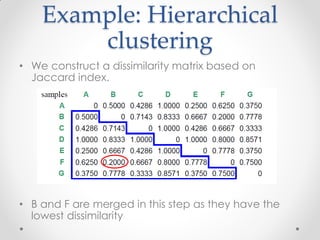
- 27. Example: Hierarchical clustering • We construct a dissimilarity matrix based on Jaccard index. • B and F are merged in this step as they have the lowest dissimilarity
- 28. Example: Hierarchical clustering • How do we calculate distance of (B,F) with other clusters? o This is where the choice of linkage criteria comes in o Since we are using complete linkage, we use the maximum distance between two clusters o So, • Dissimilarity(B, A) : 0.5000 • Dissimilarity(F, A) : 0.6250 • Hence, Dissimilarity((B,F), A) : 0.6250
- 29. Example: Hierarchical clustering • We iteratively merge clusters at each step until all the data points are covered, i. merge two clusters with lowest dissimilarity ii. update the dissimilarity matrix based on merged clusters o sfs
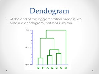
- 30. Dendogram • At the end of the agglomeration process, we obtain a dendogram that looks like this, • sfdafdfsdfsd
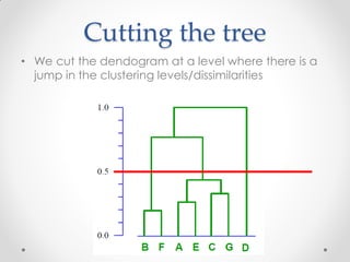
- 31. Cutting the tree • We cut the dendogram at a level where there is a jump in the clustering levels/dissimilarities
- 32. Cutting the tree • If we cut the tree at 0.5, then we can say that within each cluster the samples have more than 50% similarity • So our final set of clusters is, i. (B,F), ii. (A,E,C,G) and iii. (D)
- 33. Final set of clusters
- 34. Impact of metrics • The metrics chosen for hierarchical clustering can lead to vastly different clusters. • Distance metric o In a 2-dimensional space, the distance between the point (1,0) and the origin (0,0) can be 2 under Manhattan distance, 2 under Euclidean distance. • Linkage criteria o Distance between two clusters can be different based on linkage criteria used
- 35. Linkage criteria • Complete linkage is the most popular metric used for hierarchical clustering. It is less sensitive to outliers. • Single linkage can handle non-elliptical shapes. But, single linkage can lead to clusters that are quite heterogeneous internally and it more sensitive to outliers and noise
- 36. Pros and Cons : Hierarchical Clustering • Pros o No assumption of a particular number of clusters o May correspond to meaningful taxonomies • Cons o Once a decision is made to combine two clusters, it can’t be undone o Too slow for large data sets, O(𝑛2 log(𝑛))
- 37. References i. https://spin.atomicobject.com/2015/05/26/mean- shift-clustering/ ii. http://vision.stanford.edu/teaching/cs131_fall1314 _nope/lectures/lecture13_kmeans_cs131.pdf iii. http://84.89.132.1/~michael/stanford/maeb7.pdf
- 38. Thank you!


