SINGLE-SOURCE SHORTEST PATHS

Prepared by
Md. Shafiuzzaman
Lecturer, Dept. of CSE, JUST
SINGLE-SOURCE SHORTEST PATHS

Md. Shafiuzzaman 2
Shortest Path
Shortest Path = Path of minimum weight
δ(u,v)= min{ω(p) : u v}; if there is a path from u to v,
 otherwise.
p

Md. Shafiuzzaman 3
Shortest-Path Variants
• Shortest-Path problems
– Single-source shortest-paths problem: Find the shortest path from s
to each vertex v. (e.g. BFS)
– Single-destination shortest-paths problem: Find a shortest path to a
given destination vertex t from each vertex v.
– Single-pair shortest-path problem: Find a shortest path from u to v
for given vertices u and v.
– All-pairs shortest-paths problem: Find a shortest path from u to v
for every pair of vertices u and v.

Md. Shafiuzzaman 4
Negative-weight edges
• No problem, as long as no negative-weight cycles are
reachable from the source
• Otherwise, we can just keep going around it, and
get w(s, v) = −∞ for all v on the cycle.

Md. Shafiuzzaman 5
Relaxation
• Maintain d[v] for each v  V
• d[v] is called shortest-path weight estimate
and it is upper bound on δ(s,v)
INIT(G, s)
for each v  V do
d[v] ← ∞
π[v] ← NIL
d[s] ← 0

Md. Shafiuzzaman 6
Relaxation
RELAX(u, v)
if d[v] > d[u]+w(u,v) then
d[v] ← d[u]+w(u,v)
π[v] ← u
5
u v
vu
2
2
9
5 7
Relax(u,v)
5
u v
vu
2
2
6
5 6

Md. Shafiuzzaman 7
Properties of Relaxation
Algorithms differ in
 how many times they relax each edge, and
 the order in which they relax edges
Question: How many times each edge is relaxed in BFS?
Answer: Only once!

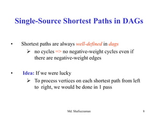
Md. Shafiuzzaman 8
Single-Source Shortest Paths in DAGs
• Shortest paths are always well-defined in dags
 no cycles => no negative-weight cycles even if
there are negative-weight edges
• Idea: If we were lucky
 To process vertices on each shortest path from left
to right, we would be done in 1 pass

Md. Shafiuzzaman 9
In a dag:
• Every path is a subsequence of the topologically sorted
vertex order
• If we do topological sort and process vertices in that order
• We will process each path in forward order
 Never relax edges out of a vertex until have processed
all edges into the vertex
• Thus, just 1 pass is sufficient

Md. Shafiuzzaman 16
DAG-SHORTEST PATHS(G, s)
TOPOLOGICALLY-SORT the vertices of G
INIT(G, s)
for each vertex u taken in topologically sorted order do
for each v  Adj[u] do
RELAX(u, v)

Md. Shafiuzzaman 17
Runs in linear time: Θ(V+E)
 topological sort: Θ(V+E)
 initialization: Θ(V+E)
 for-loop: Θ(V+E)
each vertex processed exactly once
=> each edge processed exactly once: Θ(V+E)

Md. Shafiuzzaman 18
• Non-negative edge weight
• Like BFS: If all edge weights are equal, then use BFS,
otherwise use this algorithm
• Use Q = priority queue keyed on d[v] values
(note: BFS uses FIFO)
Dijkstra’s Algorithm For Shortest Paths

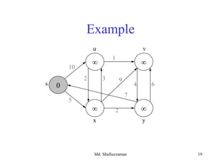
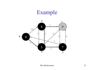
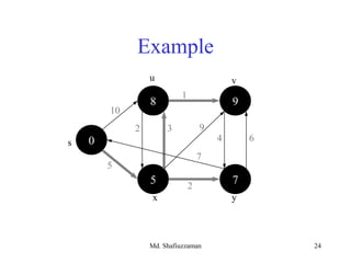
Md. Shafiuzzaman 19
Example
3
 
 
0s
u v
yx
10
5
1
2 9
4 6
7
2

Md. Shafiuzzaman 20
Example
2
10 
5 
0s
u v
yx
10
5
1
3
9
4 6
7
2

Md. Shafiuzzaman 21
Example
2
8 14
5 7
0s
yx
10
5
1
3 9
4 6
7
2
u v

Md. Shafiuzzaman 22
Example
10
8 13
5 7
0s
u v
yx
5
1
2 3 9
4 6
7
2

Md. Shafiuzzaman 23
Example
8
u v
9
5 7
0
yx
10
5
1
2 3 9
4 6
7
2
s

Md. Shafiuzzaman 24
Example
u
5
8 9
5 7
0
v
yx
10
1
2 3 9
4 6
7
2
s

Md. Shafiuzzaman 25
DIJKSTRA(G, s)
INIT(G, s)
S←Ø > set of discovered nodes
Q←V[G]
while Q ≠Ø do
u←EXTRACT-MIN(Q)
S←S U {u}
for each v  Adj[u] do
RELAX(u, v) > May cause
> DECREASE-KEY(Q, v, d[v])

Md. Shafiuzzaman 26
Observe :
• Each vertex is extracted from Q and inserted into S
exactly once
• Each edge is relaxed exactly once
• S = set of vertices whose final shortest paths have already
been determined
 i.e. , S = {v  V: d[v] = δ(s, v) ≠ ∞ }

Md. Shafiuzzaman 27
• Similar to BFS algorithm: S corresponds to the set of
black vertices in BFS which have their correct breadth-
first distances already computed
• Greedy strategy: Always chooses the closest(lightest)
vertex in Q = V-S to insert into S
• Relaxation may reset d[v] values thus updating
Q = DECREASE-KEY operation.

Md. Shafiuzzaman 28
• Similar to Prim’s MST algorithm: Both algorithms
use a priority queue to find the lightest vertex outside a
given set S
• Insert this vertex into the set
• Adjust weights of remaining adjacent vertices outside the
set accordingly

Md. Shafiuzzaman 29
Example: Run algorithm on a sample graph
43
210
5 1
s0
∞ 5
∞ 10 9 8
∞ 6

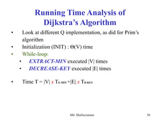
Md. Shafiuzzaman 30
• Look at different Q implementation, as did for Prim’s
algorithm
• Initialization (INIT) : Θ(V) time
• While-loop:
• EXTRACT-MIN executed |V| times
• DECREASE-KEY executed |E| times
• Time T = |V| x TE-MIN +|E| x TD-KEY
Running Time Analysis of
Dijkstra’s Algorithm

Md. Shafiuzzaman 31
Bellman-Ford Algorithm for Single
Source Shortest Paths
• More general than Dijkstra’s algorithm:
 Edge-weights can be negative
• Detects the existence of negative-weight cycle(s)
reachable from s.

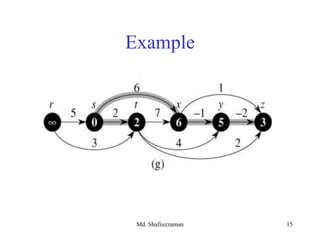
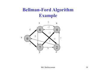
Md. Shafiuzzaman 32
Bellman-Ford Algorithm
Example
5
 
 
0s
zy
6
7
8
-3
7
2
9
-2
xt
-4

Md. Shafiuzzaman 33
Example
6 
7 
0s
zy
6
7
8
-3
7
2
9
-2
xt
-4
5

Md. Shafiuzzaman 34
Example
6 4
7 2
0s
zy
6
7
8
-3
7
2
9
-2
xt
-4
5

Md. Shafiuzzaman 35
Example
2 4
7 2
0s
zy
6
7
8
-3
7
2
9
-2
xt
-4
5

Md. Shafiuzzaman 36
Example
2 4
7 -2
0s
zy
6
7
8
-3
7
2
9
-2
xt
-4
5

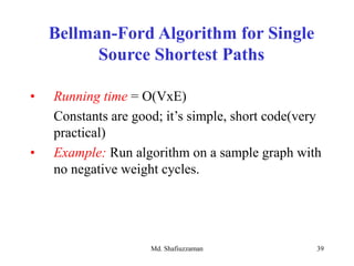
Md. Shafiuzzaman 37
BELMAN-FORD( G, s )
INIT( G, s )
for i ←1 to |V|-1 do
for each edge (u, v)  E do
RELAX( u, v )
for each edge ( u, v )  E do
if d[v] > d[u]+w(u,v) then
return FALSE > neg-weight cycle
return TRUE

Md. Shafiuzzaman 38
Observe:
• First nested for-loop performs |V|-1 relaxation passes;
relax every edge at each pass
• Last for-loop checks the existence of a negative-weight
cycle reachable from s

Md. Shafiuzzaman 39
• Running time = O(VxE)
Constants are good; it’s simple, short code(very
practical)
• Example: Run algorithm on a sample graph with
no negative weight cycles.

Md. Shafiuzzaman 40
• Converges in just 2 relaxation passes
• Values you get on each pass & how early converges
depend on edge process order
• d value of a vertex may be updated more than once in a
pass

Assignment
• Implement Dijkstra’s Algorithm and
Bellman–Ford Algorithm
• Input: Take number of vertices, adjacency
matrix and starting node as input
• Output: Print distance from each node and
the path
Md. Shafiuzzaman 41

SINGLE-SOURCE SHORTEST PATHS

More Related Content

SINGLE-SOURCE SHORTEST PATHS