Social networks, activities, and travel - building links to understand behaviour

www.its.leeds.ac.uk/people/c.calastri Social networks, i.e. the circles of people we are socially connected to, have been recognised to play a role in shaping our travel and activity behaviour. This not only has to do with socialisation being the purpose of travel, but also with enabling mobility and other activities through the so-called social capital. Another theme in the literature connecting social environment and travel behaviour is social influence, i.e. the investigation of how travel behaviour can be affected by observation or comparison with other people. Research about the impact of social influence on travel choices is still at its infancy. In this talk, I will give an overview of how choice modelling can be used to investigate the relationships between social networks, travel and activities. I will touch upon work that I have done so far, in particular I will describe my applications of the Multiple Discrete-Continuous Extreme Value (MDCEV) model to frequency of social interactions as well as to allocation of time to different activities, taking the social dimension into account. In these studies, I make use of social network and travel data collected in places as diverse as Switzerland and Chile. I will also discuss ongoing work making use of longitudinal life-course data to model the impact of family of origin and the “mobility environment” people grew up in on travel decision of adults. Finally, I will outline future plans about modelling behavioural changes due to social influence using the smartphone app travel data that are being collected in Leeds within the “Choices and consumption: modelling long and short term decisions in a changing world” (“DECISIONS”) project.


Social networks, activities, and travel - building links to understand behaviour
- 1. Social networks, activities and travel: building links to understand behaviour Chiara Calastri, Institute for Transport Studies & Choice Modelling Centre, University of Leeds
- 2. Key themes for my PhD How do people interact with their social network members, and what are the implications for travel behaviour? What is the role of personal social networks in activity patterns? Are people going to change their travel behaviour following information about themselves and other people? How are social networks formed and how do they evolve (not covered today)?
- 3. Methodological consideration Basic data analysis could give insights to answer these questions But such an approach would not be scientifically sound or satisfying to us as modellers Many factors could explain the same effect and we need to disentangle them Recent advances in choice modelling provide methodologically robust tools to deal with this A key aim of my research is to operationalise and improve these models
- 4. I – Patterns of interactions
- 5. Modelling social interactions Focus on mode and frequency of interaction Previous research mainly used multi-level models but Lack of integrated framework Did not deal with no communication No consideration of satiation
- 6. Research question How do people communicate with each of their social network members? Mode of communication (discrete choice) Frequency of communication (continuous choice)
- 7. Data: snowball sample 638 egos naming 13,500 alters, fairly representative of the Swiss population Kowald, M. (2013). Focussing on leisure travel: The link between spatial mobility, leisure acquaintances and social interactions. PhD thesis, Diss., Eidgenössische Technische Hochschule ETH Zürich, Nr. 21276, 2013.
- 9. Data:The Name Interpreter “multiple discrete-continuous choice”
- 10. Many real-life situations involve making (multiple) discrete and continuous choices at the same time In general, people will not be able to choose an unlimited amount of these goods because they have limited resources (e.g. money, time) Modelling multiple discrete-continuous choices
- 11. The Multiple Discrete-Continuous ExtremeValue (MDCEV) Model State-of-the-art approach Utility maximization-based Khun-Tucker approach demand system Desirable properties Closed form probability Based on Random Utility Maximisation Goods are imperfect substitutes and not mutually exclusive
- 12. The Multiple Discrete-Continuous ExtremeValue (MDCEV) Model Direct utility specification (Bhat, 2008): where: U(x) is the utility with respect to the consumption quantity (Kx1)-vector x (xk≥0 for all k) ψk is the baseline marginal utility, i.e. the marginal utility at zero consumption of good k 0≤αk≤1 reduces the marginal utility with increasing consumption of good k, i.e. controls satiation. If αk=1, we are in the case of constant marginal utility (MNL) γk>0 shifts the position of the indifference curves, allowing for corner solutions.
- 13. Interpretation of the ψ parameter Marginal utility of consumption w.r.t. good k ψk is the “baseline marginal utility”: utility at the point of zero consumption
- 14. Interpretation of the α parameter The alpha parameter controls satiation by exponentiating the consumption quantity. If αk=1, the person is “insatiable” with respect to good k (MNL case), while when α decreases, the consumer accrues less and less utility from additional units consumed.
- 15. Interpretation of the γ parameter The γ are translation parameters, i.e. they shift the position of indifference curves so that they intersect the axes Bhat (2005) interprets the γ parameter also as a measure of satiation because of its impact on the shape of the indifference curves Source: Bhat, Chandra R. "The multiple discrete-continuous extreme value (MDCEV) model: role of utility function parameters, identification considerations, and model extensions." TransportationResearch Part B: Methodological 42.3 (2008): 274-303.
- 16. Probabilities MDCEV allows modelling of either expenditure or consumption Model estimation maximises likelihood of observed consumption patterns by changing parameters where and Need to make assumptions about the budget
- 17. Model Specification Dependent variable: yearly frequency of communication by each mode with each network member We estimate only 4 mode-specific effects for each independent variable & satiation parameter Allocation model: individual budget given by the total annual number of interaction across all alters and all modes “Ego” “Alter”“Alter”
- 18. Results:Core parameters α1 goes to zero in all model specifications->utility collapses to a log formulation Baseline utility constants: strong baseline preference for face- to-face (interesting for the debate on ICT substitution), followed by phone Satiation (γ): Face-to-face provides more satiation, followed by phone, e-mail and SMS.
- 20. Results: dyad-level effects -1 -0.5 0 0.5 1 1.5 2 2.5 3 3.5 0 5 10 20 40 60 80 100 120 140 160 180 200 220 240 Distance f2f phone e-mail sms
- 21. Results: dyad level effects
- 22. Contact maintenance and tie strength (work in progress…)
- 23. II – Activities and social networks
- 24. Activity behaviour and social networks Activity scheduling (which, for how long, with whom,…) can provide insights into travel behaviour Existing work incorporating social environment in models of activity behaviour only focused on leisure and social activities mostly looked at one dimension of decision making mainly relied on data from the “Global North”
- 25. Activity type & duration People jointly choose to engage in different activities for certain amounts of time, e.g. to satisfy variety seeking behaviour Choice of which/how many activities to perform (e.g. in a day) not independent of duration …some of the activities might have some common unobserved characteristics -> we use the nested version of MDCEV
- 26. A nested model The MDCEV (like an MNL) assumes that all the possible correlations between alternatives is explained through the β. In some cases, some alternatives might share some unobserved correlation (estimated), so that they are closer substitutes of each other
- 27. The Multiple Discrete-Continuous Nested ExtremeValue (MDCNEV) Model The utility specification is the same as in the MDCEV model Stochastic element not anymore i.i.d. -> nested extreme value structure following the joint CDF:
- 28. The Multiple Discrete-Continuous Nested ExtremeValue (MDCNEV) Model Utility maximised subject to a time budget T We again maximise the likelihood of observing the observed time allocation across activities:
- 29. “Communities in Concepción”, Concepción (Chile) Extensive dataset collected in 2012 investigating several aspects of participants’ lives: Socio-demographic characteristics o Age o Gender o Level of education o Employment status & Job type o Family composition and characteristics o Personal and household income o Mobility tools ownership o Communication tools ownership Attitudinal questions Social network composition Activity diary for 2 full days
- 30. Time Use diary (filled in) DAY Sunday Start End What were you doing (mode) Where N° Hour Min Hour Min Street 1 Street 2 1 10 0 11 20 Wake up, breakfast Michimalongo 15 NA 2 11 20 14 0 Tidy up at home Michimalongo 15 NA 3 14 0 14 5 Going to the shop (walk) NA NA 4 14 5 14 10 In the shop Michimalongo central NA 5 14 10 14 15 Going back home (walk) NA NA 6 14 15 15 30 Lunch Michimalongo 15 NA 7 15 30 15 40 Going to a friend's home (walk) NA NA 8 15 40 15 50 At a friend's home yerbas buenas alto NA 9 15 50 16 0 Going back home (walk) NA NA 10 16 0 19 0 Stay at home Michimalongo 15 NA 11 19 0 19 30 Going to the doctor (walk) NA NA 12 19 30 21 30 Staying at the doctor Salas O’Higgins 13 21 30 22 0 Going back home (walk) NA NA 14 22 0 0 0 Stay at home, sleep Michimalongo 15 NA
- 31. ActivityClassification N Activity Description 1 Drop off- Pick Up 2 Family time to support/attend family members in non-essential activities (Helping children with homework, attending & playing w/ children) 3 Household Obligations cleaning/tiding up, taking care of pets, performing ordinary maintenance at home 4 In-home Recreation TV, internet, reading 5 Out-of-home Recreation mostly exercise and sports, cinema 6 Services medical/professional services, banking and religious 7 Social visits to/from friends and relatives and other activities 8 Shopping 9 Study school homework, University study, different type of classes, Other school and specific training. 10 Travel All the trips to/from activities. 11 Work 12 Basic needs (OUTSIDE GOOD) eat, sleep, stay home
- 32. Model specification Time allocation across 12 activities during 2 days 48 hours budget Inclusion of both socio-demographics and social network characteristics Satiation parameters are not parametrised: withgk = exp(mk ) mk = ¢fkwk where wk is a vector of individual characteristics for the kth alternative and ϕ’k is the corresponding vector of parameters.
- 33. The nesting structure More than 30 different structures attempted. Final structure: “Family” does not belong to any nest Activity Out of home -Drop off-Pick up -Out of Home recreation -Services -Shopping -Social -Travel -Work In home -Basic needs (Outside Good) -HH obligations -In-Home recreation -Study ϑin home =0.4356ϑ out of home =0.7382
- 34. In-home activities: Utility parameters Utility parameters (t-rat vs 0) Basic needs HH obligations In-home recreation Study Family Baseline constants 0 (fixed) -3.271 (-16.06) -4.682 (-16.58) -5.054 (-9.83) -5.734 (-16.44) Sex=male - -0.408 (-2.88) - - - Age<26 - - - 0.421 (1.93) - Age 26-40 - - - - - Age 40-60 - - -0.747 (-2.91) - - Lives w/partner - 0.369 (2.81) - - - Partner works - - - - - Low Income - 0.426 (3.35) - - 0.409 (1.34) 1 underage child - - - - -1.041 (-2.8) 2+ underage children - - - - 1.77 (4.56) Agüita de la Perdiz - - 0.862 (3.05) - - La Virgen - - 1.093 (3.85) - - Driving License - - - - - Internet use - - - 1.055 (2.19) - Network size - - - - - Share imm family - -1.04 (-2.96) - - - Share friends - -0.808 (-2.85) - - - Age homophily 40-60 - - - - - Share students in network - - - - - Share employed in network - - - - - Contacts 1 km dist. - - 0.413 (1.47) - - Share employed (student) - - - 4.26 (4.13) - SC children,female - - - 0.313 (1.87) - Socio-demographic effects Social network effects
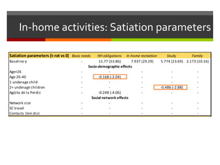
- 35. In-home activities: Satiation parameters Satiation parameters (t-rat vs 0) Basic needs HH obligations In-home recreation Study Family Baseline γ - 11.77 (53.86) 7.937 (29.29) 5.774 (23.69) 2.173 (10.16) Age<26 - - - - - Age 26-40 - -0.168 (-2.04) - - - 1 underage child - - - - - 2+ underage children - - - -0.486 (-2.88) - Agüita de la Perdiz - -0.248 (-4.06) - - - Network size - - - - - SC travel - - - - - Contacts 1km dist. - - - - - Nesting parameters (t-rat vs 1) Basic needs HH obligations In-home recreation Study Family ϑ in home 0.436 (9.54) - ϑ out of home - - - - - ϑ family (un-nested) - - - - 1 (fixed) Socio-demographic effects Social network effects
- 36. Utility parameters (t-rat vs 0) Work Drop-off/Pick-up Out-of-Home Recreation Services Social Shopping Travel Baseline constants -3.827 (-30.12) -6.133 (-14.5) -4.0542 (-25.71) -4.1466 (-34.41)-3.9735 (-8.38) -3.4295 (-15.22) -3.9229 (-4.41) Sex=male - - - - - - - Age$<$26 - - - - - - - Age 26-40 0.449 (2.87) - - - - - - Age 40-60 - - - - - - - Lives w/partner - - - - - 0.472 (2.43) - Partner works - 0.648 (2.04) - - - - - Low Income - 1.029 (3.83) - - - - - 1 underage child 0.759 (3.32) - - - - - - 2+ underage children - 1.141 (3.17) - - - - - Agüita de la Perdiz - - - - 0.259 (1.61) - - La Virgen - - - - - - - Driving License - 0.713 (2.43) - - - - - Internet use - - - - 0.402 (1.92) - - Network size - - - - 0.304 (1.85) - 1.4446 (4.45) Share imm family - - - - - - - Share friends - - - - - -0.858 (-2.48) - Age homophily 40-60 - - - - -0.657 (-2.31) - - Share students in network - - 1.244 (3.31) - - - - Share employed in network 1.426 (5.57) - - - - - - Contacts 1 km dist. - -1.838 (-2.99) -0.52 (-1.44) - - 0.861 (-2.39) -1.4028 (-2.28) Share employed (student) - - - - - - - SC children,female - 0.774 (2.83) - - - - - Socio-demographic effects Social network effects Out-of-home activities: Utility parameters
- 37. Satiation parameters (t-rat vs 0) Work Drop-off/Pick-up Out-of-Home Recreation Services Social Shopping Travel Baseline γ 5.841 (46.02) 0.344 (1.7) 2.637 (18.12) 1.659 (9.52) 2.643 (19.86) 0.8574 (6.33) 0.1695 (0.55) Age$<$26 - - - - - 0.0541 (1.55) - Age 26-40 - - - - - - - 1 underage child -0.189 (-2.92) - - - - - - 2+ underage children - - - - - - - Agüita de la Perdiz - - - - - - - Network size - - - - - - -1.3054 (-4.45) SC travel - - - - - - -0.1691 (-1.94) Contacts 1km dist. - - - - - 0.2167 (1.89) 0.2798 (1.58) Nesting parameters (t-rat vs 1) Work Drop-off/Pick-up Out-of-Home Recreation Services Social Shopping Travel ϑ in home - - - - - - - ϑ out of home ϑ family (un-nested) - - - - - - - Socio-demographic effects Social network effects 0.7382 (18.28) Out-of-home activities : Satiation parameters
- 38. Results: discrete and continuous choice Utility parameters (t-rat vs 0) Work Drop-off/Pick-up Out-of-Home Recreation Services Social Sh Baseline constants -3.827 (-30.12) -6.133 (-14.5) -4.0542 (-25.71) -4.1466 (-34.41)-3.9735 (-8.38) -3.42 Sex=male - - - - - Age$<$26 - - - - - Age 26-40 0.449 (2.87) - - - - Age 40-60 - - - - - Lives w/partner - - - - - 0.4 Partner works - 0.648 (2.04) - - - Low Income - 1.029 (3.83) - - - 1 underage child 0.759 (3.32) - - - - 2+ underage children - 1.141 (3.17) - - - Agüita de la Perdiz - - - - 0.259 (1.61) La Virgen - - - - - Driving License - 0.713 (2.43) - - - Internet use - - - - 0.402 (1.92) Network size - - - - 0.304 (1.85) Share imm family - - - - - Share friends - - - - - -0.8 Age homophily 40-60 - - - - -0.657 (-2.31) Share students in network - - 1.244 (3.31) - - Share employed in network 1.426 (5.57) - - - - Contacts 1 km dist. - -1.838 (-2.99) -0.52 (-1.44) - - 0.86 Share employed (student) - - - - - Socio-demographic effects Social network effects Satiation parameters (t-rat vs 0) Work Drop-off/Pick-up Out-of-Ho Baseline γ 5.841 (46.02) 0.344 (1.7) 2.63 Age$<$26 - - Age 26-40 - - 1 underage child -0.189 (-2.92) - 2+ underage children - - Agüita de la Perdiz - - Network size - - SC travel - - Contacts 1km dist. - - Nesting parameters (t-rat vs 1) Work Drop-off/Pick-up Out-of-Ho ϑ in home - - ϑ out of home ϑ family (un-nested) - - Socio-demogr Social netw
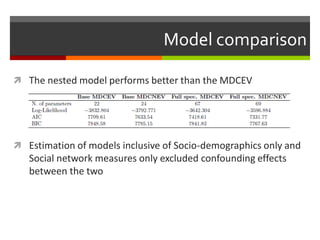
- 39. Model comparison The nested model performs better than the MDCEV Estimation of models inclusive of Socio-demographics only and Social network measures only excluded confounding effects between the two
- 40. III – Conclusions and next steps
- 41. Does our work matter? Choice modelling can really make a difference here! We gain important insights into interactions between people and the role of the social network in activities Working on methodological contributions to get further insights: Multiple budgets & product-specific upper limits on consumption Important in a multi-day context, for example Evolution of discrete and continuous elements over time We can use the models to forecast changes in activities, which have repercussions on transport demand
- 42. Our idea for an overall framework
- 43. We need complex data for this
- 44. Thank you!