Time series
- 1. Time series Analysis Amiya Kumar dash
- 2. Introduction • Time series modelling is a popular and recent area which has attracted attention of researcher community over last few decades. • The main aim of time series analysis is to collect and analyze the past observations to develop an appropriate model which can then be used to generate future values for the series, that is, to make forecasts. • The basic idea of Time series analysis is that , the history of occurrences over time can be used to predict the future. • Here, prediction of the future depends upon the past values of a variable or past error without attempting to discover the factors affecting the behavior of the series. • Time series forecasting is popularly used in several practical fields like finance, science, business, engineering and economics etc.
- 3. Uses of Time Series • The most important use of studying time series is that it helps us to predict the future behaviour of the variable based on past experience • It is helpful for business planning as it helps in comparing the actual current performance with the expected one • From time series, we get to study the past behaviour of the phenomenon or the variable under consideration • We can compare the changes in the values of different variables at different times or places, etc.
- 4. Time series Model • A time series is a sequential set of data points, measured typically at successive times. It is mathematically defined as a set of vectors X(t) . Where t= 0,1,2,….. Represents the time elapsed. The variable X(t) is a random variable. • This model generally reflects the fact that observations close together in time will be more closely related than observations further apart. • It always follow the natural-one way ordering of time, so that values for a given period will be expressed as deriving in some ways from the past values, rather than from future values.
- 5. Components for Time Series Analysis • Any time series is a composition of many individual underlying component time series. Some of these components are predictable where as other components may be almost random which can be difficult to predict. • For example a typical time series can be considered to be a combination of four components 1. Trend component 2. Cyclical component 3. Seasonal component 4. Irregular component
- 6. Components for Time Series Analysis
- 7. Trend: • The trend shows the general tendency of the data to increase or decrease during a long period of time. A trend is a smooth, general, long-term, average tendency. It is not always necessary that the increase or decrease is in the same direction throughout the given period of time. • it is defined as the “long term ” movement in a time series without calendar-related and irregular effect and is a reflection of underlying level. • It is observable that the tendencies may increase, decrease or are stable in different sections of time. But the overall trend must be upward, downward or stable. • It is the result of influences such as population growth, price inflation and general economic changes. Linear and Non-Linear Trend If we plot the time series values on a graph in accordance with time t. The pattern of the data clustering shows the type of trend. If the set of data cluster more or less round a straight line, then the trend is linear otherwise it is non-linear (Curvilinear).
- 8. Seasonal Variations These are the rhythmic forces which operate in a regular and periodic manner over a span of less than a year. They have the same or almost the same pattern during a period of 12 months. This variation will be present in a time series if the data are recorded hourly, daily, weekly, quarterly, or monthly. These variations come into play either because of the natural forces or man-made conventions. Cyclic Variations The variations in a time series which operate themselves over a span of more than one year are the cyclic variations. This oscillatory movement has a period of oscillation of more than a year. One complete period is a cycle. This cyclic movement is sometimes called the ‘Business Cycle’. Any Regular pattern of the sequence of values above and below the trend line. It is a four- phase cycle comprising of the phases of prosperity, recession, depression, and recovery. Irregular Movements They are not regular variations and are purely random or irregular. These fluctuations are unforeseen, uncontrollable, unpredictable, and are erratic. These forces are earthquakes, wars, flood, famines, and any other disasters.
- 9. Mathematical Representation of Decomposition Model for Time Series Analysis
- 10. Additive Model for Time Series Analysis Note: In some time series the amplitude of both the seasonal and irregular variations do not change as the level of trend rises or falls. In such cases additive models are appropriate
- 11. Multiplicative Model for Time Series Analysis • The multiplicative model assumes that the various components in a time series operate proportionately to each other. According to this model yt = Tt × St × Ct × Rt • Multiplicative model implies components are interactive. It is more prevalent with economic series since most seasonal economic series have a seasonal variation which increases with the level of the series.
- 12. Averaging Model
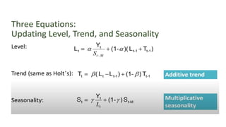
- 13. Exponential smoothing model • It is an extension to moving average (weighted MA) • It assumes that more recent values of the series will contribute more information to the forecast of the next value. • So, while forecasting the future observations, put greater weight on the most recent observations. • The class of exponential smoothing methods consists of a range of techniques as follows Simple Exponential Smoothing Holt’s Method Holt-Winters’ Method
- 17. Holt-Winters Methods • It is also known as Advanced Exponential smoothing. Also called as “Triple exponential smoothing” • The idea is to extend the simple exponential smoothing to capture the trend and/or seasonality • Applicable for data where we need to forecast a series with trend and/or seasonality • Advantage: popular and cheap to compute
- 19. • Augment Holt’s method by capturing the seasonal component Forecast= estimated Level + Trend + seasonality at most recent time point
- 20. • Two Holt-Winters methods are designed for time series that exhibit linear trend - Additive Holt-Winters method: used for time series with constant (additive) seasonal variations • Multiplicative Holt-Winters method: used for time series with increasing (multiplicative) seasonal variations
- 23. What exactly is an ARIMA model? • ARIMA, short for ‘Auto Regressive Integrated Moving Average’ is actually a class of models that ‘explains’ a given time series based on its own past values, that is, its own lags and the lagged forecast errors, so that equation can be used to forecast future values. • Any ‘non-seasonal’ time series that exhibits patterns and is not a random white noise can be modeled with ARIMA models. • An ARIMA model is characterized by 3 terms: p, d, q where, p is the order of the AR term q is the order of the MA term d is the number of differencing required to make the time series stationary
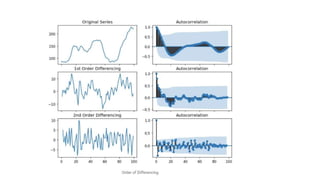
- 24. What does the p, d and q in ARIMA model mean • Term ‘Auto Regressive’ in ARIMA means it is a linear regression model that uses its own lags as predictors. Linear regression models, as you know, work best when the predictors are not correlated and are independent of each other. So how to make a series stationary? • The most common approach is to difference it. That is, subtract the previous value from the current value. Sometimes, depending on the complexity of the series, more than one differencing may be needed. • The value of d, therefore, is the minimum number of differencing needed to make the series stationary. And if the time series is already stationary, then d = 0. • ‘p’ is the order of the ‘Auto Regressive’ (AR) term. It refers to the number of lags of Y to be used as predictors. And ‘q’ is the order of the ‘Moving Average’ (MA) term. It refers to the number of lagged forecast errors that should go into the ARIMA Model.
- 25. What are AR and MA models • A pure Auto Regressive (AR only) model is one where 𝑦𝑡 depends only on its own lags. That is, 𝑦𝑡 is a function of the ‘lags of 𝑦𝑡’. Where 𝑦𝑡−1 is the lag1 of the series and β1 is the coefficient of lag1 that the model estimates and α is the intercept term, also estimated by the model. • Likewise a pure Moving Average (MA only) model is one where 𝑦𝑡 depends only on the lagged forecast errors.
- 27. How to determine the right order of differencing? • The right order of differencing is the minimum differencing required to get a near-stationary series which roams around a defined mean and the ACF plot reaches to zero fairly quick. • If the autocorrelations are positive for many number of lags (10 or more), then the series needs further differencing. On the other hand, if the lag 1 autocorrelation itself is too negative, then the series is probably over-differenced. • you need differencing only if the series is non-stationary. Else, no differencing is needed, that is, d=0.
- 30. References • Data Analytics, Radha Shankarmani, M. Vijayalaxmi, Wiley India Private Limited, ISBN: 9788126560639. • Data Science and Big Data Analytics: Discovering, Analyzing, Visualizing and Presenting Data by EMC Education Services (Editor), Wiley, 2014


