timeseries cheat sheet with example code for R
- 1. Time Series Forecasting with Python – Cheat Sheet Data Science with Marco ACF plot The autocorrelation function (ACF) plot shows the autocorrelation coefficients as a function of the lag. • Use it to determine the order q of a stationary MA(q) process • A stationary MA(q) process has significant coefficients up until lag q Output for a MA(2) process (i.e., q = 2): Time series analysis PACF plot The partial autocorrelation function (PACF) plot shows the partial autocorrelation coefficients as a function of the lag. • Use it to determine the order p of a stationary AR(p) process • A stationary AR(p) process has significant coefficients up until lag p Output for an AR(2) process (i.e., p = 2): Time series decomposition Separate the series into 3 components: trend, seasonality, and residuals • Trend: long-term changes in the series • Seasonality: periodical variations in the series • Residuals: what is not explained by trend and seasonality Note: m is the frequency of data (i.e., how many observations per season)
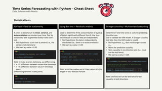
- 2. Time Series Forecasting with Python – Cheat Sheet Data Science with Marco ADF test – Test for stationarity A series is stationary it its mean, variance, and autocorrelation are constant over time. Test for stationarity with augmented Dickey-Fuller (ADF) test. • Null hypothesis: a unit root is present (i.e., the series is not stationary) • We want a p-value < 0.05 Note: to make a series stationary, use differencing. • n = 1: difference between consecutive timesteps • n = 4: difference between values 4 timesteps apart Differencing removes n data points. Statistical tests Ljung-Box test – Residuals analysis Used to determine if the autocorrelation of a group of data is significantly different from 0. Use it on the residuals to check if they are independent. • Null hypothesis: the data is independently distributed (i.e., there is no autocorrelation) • We want a p-value > 0.05 Note: print the p-values up to h lags, where h is the length of your forecast horizon Granger causality – Multivariate forecasting Determine if one time series is useful in predicting the other one. Use to validate the VAR model. If Granger causality test fails, then the VAR model is invalid. • Null hypothesis: 𝑦2,𝑡 does not Granger-causes 𝑦1,𝑡 • Works for predictive causality • Tests causality in one direction only (i.e., must run the test twice) • We want a p-value < 0.05 Note: see how we run the test twice to test causality in both directions
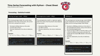
- 3. Time Series Forecasting with Python – Cheat Sheet Data Science with Marco Moving average model – MA(q) The moving average model: the current value depends on the mean of the series, the current error term, and past error terms. • Denoted as MA(q) where q is the order • Use ACF plot to find q • Assumes stationarity. Use only on stationary data Equation 𝑦𝑡 = 𝜇 + 𝜖𝑡 + 𝜃1𝜖𝑡−1 + 𝜃2𝜖𝑡−2 + ⋯ + 𝜃𝑞𝜖𝑡−𝑞 Forecasting – Statistical models Autoregressive model – AR(p) The autoregressive model is a regression against itself. This means that the present value depends on past values. • Denoted as AR(p) where p is the order • Use PACF to find p • Assumes stationarity. Use only on stationary data Equation 𝑦𝑡 = 𝐶 + 𝜙1𝑦𝑡−1 + 𝜙2𝑦𝑡−2 + ⋯ + 𝜙𝑝𝑦𝑡−𝑝 + 𝜖𝑡 ARMA(p,q) The autoregressive moving average model (ARMA) is the combination of the autoregressive model AR(p), and the moving average model MA(q). • Denoted as ARMA(p,q) where p is the order of the autoregressive portion, and q is the order of the moving average portion • Cannot use ACF or PACF to find the order p, and q. Must try different (p,q) value and select the model with the lowest AIC (Akaike’s Information Criterion) • Assumes stationarity. Use only on stationary data. Equation 𝑦𝑡 = 𝐶 + 𝜙1𝑦𝑡−1 + ⋯ 𝜙𝑝𝑦𝑡−𝑝 + 𝜃1𝜖𝑡−1 + ⋯ 𝜃𝑞𝜖𝑡−𝑞 + 𝜖𝑡
- 4. Time Series Forecasting with Python – Cheat Sheet Data Science with Marco ARIMA(p,d,q) The autoregressive integrated moving average (ARIMA) model is the combination of the autoregressive model AR(p), and the moving average model MA(q), but in terms of the differenced series. • Denoted as ARMA(p,d,q), where p is the order of the autoregressive portion, d is the order of integration, and q is the order of the moving average portion • Can use on non-stationary data Equation 𝑦′𝑡 = 𝐶 + 𝜙1𝑦′𝑡−1 + ⋯ 𝜙𝑝𝑦′𝑡−𝑝 + 𝜃1𝜖𝑡−1 + ⋯ 𝜃𝑞𝜖𝑡−𝑞 + 𝜖𝑡 Note: the order of integration d is simply the number of time a series was differenced to become stationary. Forecasting – Statistical models SARIMA(p,d,q)(P,D,Q)m The seasonal autoregressive integrated moving average (SARIMA) model includes a seasonal component on top of the ARIMA model. • Denoted as SARIMA(p,d,q)(P,D,Q)m. Here, p, d, and q have the same meaning as in the ARIMA model. • P is the seasonal order of the autoregressive portion • D is the seasonal order of integration • Q is the seasonal order of the moving average portion • m is the frequency of the data (i.e., the number of data points in one season) SARIMAX SARIMAX is the most general model. It combines seasonality, a moving average portion, an autoregressive portion, and exogenous variables. • Can use external variables to forecast a series Caveat: SARIMAX predicts the next timestep. If your horizon is longer than one timestep, then you must forecast your exogenous variables too, which can amplify the error in your model
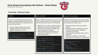
- 5. Time Series Forecasting with Python – Cheat Sheet Data Science with Marco VARMAX The vector autoregressive moving average with exogenous variables (VARMAX) model is used for multivariate forecasting (i.e., predicting two time series at the same time) • Assumes Granger-causality. Must use the Granger-causality test. If the test fails, the VARMAX model cannot be used. Forecasting – Statistical models BATS and TBATS BATS and TBATS are used when the series has more than one seasonal period. This can happen when we have high frequency data, such as daily data. • When there is more than one seasonal period, SARIMA cannot be used. Use BATS or TBATS. • BATS: Box-Cox transformation, ARMA errors, Trend and Seasonal components • TBATS: Trigonometric seasonality, Box-Cox transformation, ARMA errors, Trend and Seasonal components. Exponential smoothing Exponential smoothing uses past values to predict the future, but the weights decay exponentially as the values go further back in time. • Simple exponential smoothing: returns flat forecasts • Double exponential smoothing: adds a trend component. Forecasts are a straight line (increasing or decreasing) • Triple exponential smoothing: adds a seasonal component • Trend can be “additive” or “exponential” • Seasonality can be “additive” or “multiplicative”
- 6. Time Series Forecasting with Python – Cheat Sheet Data Science with Marco Deep neural network (DNN) A deep neural network stacks fully connected layers and can model non-linear relationship in the time series if the activation function is non-linear. • Start with a simple model with few hidden layers. Experiment training for more epochs before adding layers Forecasting – Deep learning models Long short-term memory - LSTM An LSTM is great at processing sequences of data, such as text and time series. Its architecture allows for past information to still be used for later predictions • You can stack many LSTM layers in your model • You can try combining an LSTM with a CNN • An LSTM is longer to train since the data is processed in sequence Convolutional neural network - CNN A CNN can act as a filter for our time series, due to the convolution operation which reduces the feature space. • A CNN trains faster than an LSTM • Can be combined with an LSTM. Place the CNN layer before the LSTM
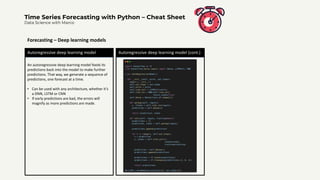
- 7. Time Series Forecasting with Python – Cheat Sheet Data Science with Marco Autoregressive deep learning model An autoregressive deep learning model feeds its predictions back into the model to make further predictions. That way, we generate a sequence of predictions, one forecast at a time. • Can be used with any architecture, whether it’s a DNN, LSTM or CNN • If early predictions are bad, the errors will magnify as more predictions are made. Forecasting – Deep learning models Autoregressive deep learning model (cont.)


