Unit 8 searching and hashing

Searching and Hashing
1
By:
Dabal Singh Mahara
2017

Unit – 8 Searching and Hashing
Contents Hours Marks
• Introduction
• Sequential search
• Binary search
• Comparison and efficiency of searching
• Hashing
 probing (Linear and Quadratic)
5 7
2

3
Introduction
• Searching is a process of finding an element within the list of
elements stored in any order or randomly.
• Searching is divided into two categories Linear and Binary search.
• Linear search
 Small arrays
 Unsorted arrays
• Binary search
 Large arrays
 Sorted arrays

4
• In linear search, access each element of an array one by one sequentially and see whether it
is desired element or not. A search will be unsuccessful if all the elements are accessed and
the desired element is not found.
• In brief, Simply search for the given element left to right and return the index of the
element, if found. Otherwise return “Not Found”.
Algorithm:
LinearSearch(A, n,key)
{
for(i=0;i<n;i++)
{
if(A[i] == key)
return i;
}
return -1; //-1 indicates unsuccessful search
}
Analysis: Time complexity = O(n)
Linear Search

5
Binary Search
• Binary search is an extremely efficient algorithm.
• This search technique searches the given item in minimum possible comparisons.
• To do this binary search, first we need to sort the a elements.
• The logic behind this technique is given below:
i. First find the middle element of the array
ii. Compare the middle element with an item.
iii. There are three cases:
a. If it is a desired element then search is successful
b. If it is less than desired item then search only the first half of the array.
c. If it is greater than the desired element, search in the second half of
the array.
• Repeat the same process until element is found or exhausts in the search area.
• In this algorithm every time we are reducing the search area.

6
Iterative Algorithm
BinarySearch(A, l, r, key)
{
while(l<=r)
{
m = (l + r) /2 ; //integer division
if(key = = A[m]
print " Search successful"
else if (key < A[m])
r = m - 1
else
l = m+1
}
If(l>r)
print "unsuccessful search"
}

7
BinarySearch(A, l, r, key)
{
if(l= = r) //only one element
{
if(key = = A[l])
print " successful Search"
else
print "unsuccessful Search"
}
else
{
m = (l + r) /2 ; //integer division
if(key = = A[m]
print "successful search"
else if (key < A[m])
return BinarySearch(A, l, m-1, key) ;
else
return BinarySearch(A, m+1, r, key) ;
}
}
Algorithm: Recursive

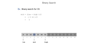
8
Binary Search Example
• Ex. Binary search for 33.
641413 25 33 5143 53 8472 93 95 97966
low high

821 3 4 65 7 109 11 12 14130
641413 25 33 5143 53 8472 93 95 97966
Binary Search
low
Ex. Binary search for 33.
low = 0
high = 14
high

Binary Search
mid = (low + high)/2
= ( 0 + 14 )/2
= 7
821 3 4 65 7 109 11 12 14130
641413 25 33 5143 53 8472 93 95 97966
low highmid

Binary Search
821 3 4 65 7 109 11 12 14130
641413 25 33 5143 53 8472 93 95 97966
low high
Since key < A [mid],
Update: high = mid -1
Low = 0
High = 6

Binary Search
mid = (low + high )/2
= ( 0 +6 )/2
= 3
821 3 4 65 7 109 11 12 14130
641413 25 33 5143 53 8472 93 95 97966
low mid high

Binary Search
821 3 4 65 7 109 11 12 14130
641413 25 33 5143 53 8472 93 95 97966
low high
Since key > A [mid],
Update: low = mid +1

Binary Search
821 3 4 65 7 109 11 12 14130
641413 25 33 5143 53 8472 93 95 97966
low highmid
mid = (low + high )/2
= ( 4 +6 )/2
= 5

Binary Search
821 3 4 65 7 109 11 12 14130
641413 25 33 5143 53 8472 93 95 97966
low
high
Since key < A [mid],
Update: low = mid -1

Binary Search
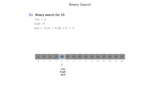
low = 4
high =4
mid = (low + high )/2 = 4
821 3 4 65 7 109 11 12 14130
641413 25 33 5143 53 8472 93 95 97966
low
high
mid

Binary Search
a[mid] = 33
search successful !!
821 3 4 65 7 109 11 12 14130
641413 25 33 5143 53 8472 93 95 97966
low
high
mid

18
Trace Binary Search
Take input array a[]
For Search key = 2
l r mid remarks
0 13 6 Key < a[6] i.e. 2 < 53
0 5 2 Key < a[2] i.e. 2 < 7
0 1 0 Key == a[0] i.e. 2 ==a[0]
Therefore, key found at index 0.
Search Successful !!
2 5 7 9 18 45 53 59 67 72 88 95 101 104
0 1 2 3 4 5 6 7 8 9 10 11 12 13
Exercise : Trace binary search algorithm for keys:
i. 67
ii. 50
iii. 250

19
Search for key = 67
l r mid Remarks
0 13 6 Key < a[6] i.e. 67 > 53
7 13 10 Key < a[10] i.e. 67 < 88
7 9 8 Key == a[8] i.e. 67 ==a[8]
Therefore, key found at index 8.
Search Successful !!
2 5 7 9 18 45 53 59 67 72 88 95 101 104
0 1 2 3 4 5 6 7 8 9 10 11 12 13
Input Array : a[ ]

20
Search for key = 50
l r mid Remarks
0 13 6 Key < a[6] i.e. 50 < 53
0 5 2 Key < a[2] i.e. 50 > 7
3 5 4 Key > a[4] i.e. 50 >18
5 5 5 Key > a[5] i.e. 50 > 45
6 5 l > r, terminate
Therefore, key not found in the array.
Search Unsuccessful !!
2 5 7 9 18 45 53 59 67 72 88 95 101 104
0 1 2 3 4 5 6 7 8 9 10 11 12 13
Given Input Array a[]

21
Efficiency:
From the above algorithm we can say that the running time of the
algorithm is:
T(n) = T(n/2) + Ο(1)
= Ο(log n)
 In the best case output is obtained at one run
i.e. Ο(1) time if the key is at middle.
 In the worst case the output is at the end of the array,
So running time is Ο(log n)
 In the average case also running time is Ο(log n).

22
Introduction to Hashing
• Suppose that we want to store 10,000 students records (each with a 5-digit ID) in a
given container.
 A linked list implementation would take O(n) time.
 A height balanced tree would give O(log n) access time.
 Using an array of size 100,000 would give O(1) access time but will lead
to a lot of space wastage.
• Is there some way that we could get O(1) access without wasting a lot of space?
• The answer is hashing.

23
Introduction to Hashing
 Hashing is a technique used for performing insertions, deletions and
finds in constant average time O(1).
 The techniques employed here is to compute location of desired
record to retrieve it in a single access or comparison.
 This data structure, however, is not efficient in operations that
require any ordering information among the elements, such as
findMin, findMax and printing the entire table in sorted order.
Applications
• Database systems
• Symbol table for compilers
• Data Dictionaries
• Browser caches

24
 The ideal hash table structure is an array of some fixed size,
containing the items.
 A stored item needs to have a data member, called key, that will be
used in computing the index value for the item.
• Key could be an integer, a string, etc
e.g. a name or Id that is a part of a large employee structure
 The size of the array is TableSize.
 The items that are stored in the hash table are indexed by values from
0 to TableSize – 1.
 Each key is mapped into some number in the range 0 to TableSize – 1.
 The mapping is called a hash function.
Hash Table

25
Example
Hash
Function
mary 28200
dave 27500
phil 31250
john 25000
Items
Hash
Table
key
key
0
1
2
3
4
5
6
7
8
9
mary 28200
dave 27500
phil 31250
john 25000

26
Hash Functions (cont’d)
• A hash function, h, is a function which transforms a key from a set, K,
into an index in a table of size n:
h: K -> {0, 1, ..., n-2, n-1}
• A key can be a number, a string, a record etc.
• The size of the set of keys, |K|, to be relatively very large.
• It is possible for different keys to hash to the same array location. This
situation is called collision and the colliding keys are called synonyms.
• A common hash function is
h(x)=x mod SIZE
• if key=27 and SIZE=10 then
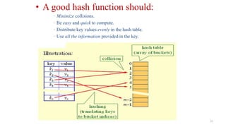
hash address=27%10=7

27
• A good hash function should:
· Minimize collisions.
· Be easy and quick to compute.
· Distribute key values evenly in the hash table.
· Use all the information provided in the key.

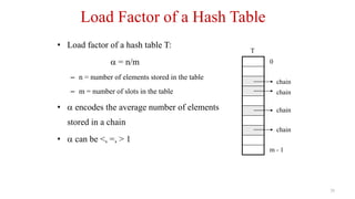
28
Load Factor of a Hash Table
• Load factor of a hash table T:
 = n/m
– n = number of elements stored in the table
– m = number of slots in the table
•  encodes the average number of elements
stored in a chain
•  can be <, =, > 1
0
m - 1
T
chain
chain
chain
chain

29
Collision Resolution
• If, when an element is inserted, it hashes to the same value as an already
inserted element, then we have a collision and need to resolve it.
i.e. For any two keys k1 and k2,
H(k1) = H(k2) = β
• There are several methods for dealing with this:
– Separate chaining
– Open addressing
• Linear Probing
• Quadratic Probing
• Double Hashing

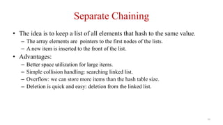
30
Separate Chaining
• The idea is to keep a list of all elements that hash to the same value.
– The array elements are pointers to the first nodes of the lists.
– A new item is inserted to the front of the list.
• Advantages:
– Better space utilization for large items.
– Simple collision handling: searching linked list.
– Overflow: we can store more items than the hash table size.
– Deletion is quick and easy: deletion from the linked list.

31
Example
0
1
2
3
4
5
6
7
8
9
0
81 1
64 4
25
36 16
49 9
Keys: 0, 1, 4, 9, 16, 25, 36, 49, 64, 81
hash(key) = key % 10.
Exercise: Represent the keys {89, 18, 49, 58, 69, 78} in
hash table using separate chaining.

32
Operations
• Initialization: all entries are set to NULL
• Find:
– locate the cell using hash function.
– sequential search on the linked list in that cell.
• Insertion:
– Locate the cell using hash function.
– (If the item does not exist) insert it as the first item in
the list.
• Deletion:
– Locate the cell using hash function.
– Delete the item from the linked list.

33
Collision Resolution with
Open Addressing
• Separate chaining has the disadvantage of using linked lists.
– Requires the implementation of a second data structure.
• In an open addressing hashing system, all the data go inside the table.
– Thus, a bigger table is needed.
• Generally the load factor should be below 0.5.
– If a collision occurs, alternative cells are tried until an empty cell is found.

34
Open Addressing
• More formally:
– Cells h0(x), h1(x), h2(x), …are tried in succession
where, hi(x) = (hash(x) + f(i)) mod TableSize, with f(0) = 0.
– The function f is the collision resolution strategy.
• There are three common collision resolution strategies:
– Linear Probing
– Quadratic probing
– Double hashing

35
Linear Probing
• In linear probing, collisions are resolved by sequentially
scanning an array (with wraparound) until an empty cell is
found.
• hi(x) = (hash(x) + f(i)) mod TableSize
– i.e. f is a linear function of i, typically f(i)= i.
 Example: Insert keys {89, 18, 49, 58, 69, 78} with the hash
function: h(x)=x mod 10 using linear probing. Use table size
10.
 when x=89:
h(89)=89%10=9
insert key 89 in hash-table in location 9
 when x=18:
h(18)=18%10=8

36
when x=49:
h(49)=49%10=9 (Collision )
so insert key 49 in hash-table in next
possible vacant location of 9 is 0
 when x=58:
h(58)=58%10=8 (Collision)
insert key 58 in hash-table in next
(since 9, 0 already contains values).
 when x=69:
h(89)=69%10=9 (Collision )
insert key 69 in hash-table in next
(since 0, 1 already contains values).
 when x = 78
h(78) = 78 % 10 = 8 ( Collision )
search next vacant slot in the table
which is 3 (since 0,1,2 contain values)
insert 78 at location 3.
0 49
1 58
2 69
3 78
4
5
6
7
8 18
9 89
Fig. Hash table with keys
Using linear probing

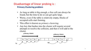
37
Disadvantage of linear probing is :
Primary Clustering problem
• As long as table is big enough, a free cell can always be
found, but the time to do so can get quite large.
• Worse, even if the table is relatively empty, blocks of
occupied cells start forming.
• This effect is known as primary clustering.
• Any key that hashes into the cluster will require several
attempts to resolve the collision, and then it will add to the
cluster.

38
 Quadratic probing is a collision resolution method that eliminates the
primary clustering problem take place in a linear probing.
 Compute: Hash value = h(x) = x % table size
 When collision occur then the quadratic probing works as follows:
(Hash value + 12)% table size,
 if there is again collision occur then there exist rehashing.
(hash value + 22)%table size
 if there is again collision occur then there exist rehashing.
(hash value = 32)% table size
 In general in ith collision
hi(x)=(hash value +i2)%size
Quadratic Probing:

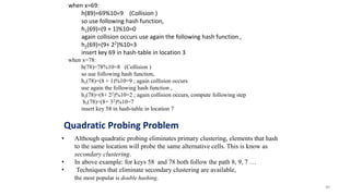
39
solution:
when x=89:
h(89)=89%10=9
when x=18:
h(18)=18%10=8
when x=49:
h(49)=49%10=9 (Collision )
so use following hash function,
h1(49)=(9 + 1)%10=0
hence insert key 49 in hash-table in location 0
when x=58:
h(58)=58%10=8 (Collision )
h1(58)=(8 + 1)%10=9
again collision occur use again the following hash function ,
h2(58)=(8+ 22)%10=2
Example: Insert keys {89, 18, 49, 58, 69 78} with the hash-table size 10 using
quadratic probing.
0 49
1
2 58
3 69
4
5
6
7 78
8 18
9 89
Using quadratic probing

40
when x=69:
h(89)=69%10=9 (Collision )
h1(69)=(9 + 1)%10=0
again collision occurs use again the following hash function ,
h2(69)=(9+ 22)%10=3
when x=78:
h(78)=78%10=8 (Collision )
h1(78)=(8 + 1)%10=9 ; again collision occurs
use again the following hash function ,
h2(78)=(8+ 22)%10=2 ; again collision occurs, compute following step
h3(78)=(8+ 32)%10=7
• Although quadratic probing eliminates primary clustering, elements that hash
to the same location will probe the same alternative cells. This is know as
secondary clustering.
• In above example: for keys 58 and 78 both follow the path 8, 9, 7 …
• Techniques that eliminate secondary clustering are available,
the most popular is double hashing.
Quadratic Probing Problem

41
Double Hashing
 To eliminate both types of clustering one way is double hashing.
 It involves two hash functions, h1(x) and h2(x),
where h1(x) is primary hash function, is first used to determine position of
key and if it is occupied h2(x) is used.
 Example: h1(x) = x % TABLESIZE
h2(x) = R – (x % R), Where R is prime less than table size
hi(x) = h1 (x) + i.h2(x) ) % TABLESIZE
 Example: Insert keys {89, 18, 49, 58, 69 78} with the hash-
table size 10 using double hashing.
solution:
 when x=89:
h(89)=89%10=9
 when x=18:
h(18)=18%10=8

42
 when x=49:
h(49)=49%10=9 (Collision )
h1(49)=(9 + 1(7- 49%7))%10
= (9 + (7-0) ) % 10
= 6
hence insert key 49 in hash-table in location 6.
 when x=58:
h(58)=58%10=8 (Collision )
h1(58) = (8 + 1(7-(58%7))%10
=(8 + (7-2))% 10
=3
INSERT 58 in the location 3.
Compute the location for keys:
 69
 78
0
1
2
3 58
4
5
6 49
7
8 18
9 89
Using double hashing
Limitation:
It takes extra time to compute hash function.

Unit 8 searching and hashing

More Related Content

Unit 8 searching and hashing