
Abstract
Understanding how biological neural networks carry out learning using spike-based local plasticity mechanisms can lead to the development of real-time, energy-efficient, and adaptive neuromorphic processing systems. A large number of spike-based learning models have recently been proposed following different approaches. However, it is difficult to assess if these models can be easily implemented in neuromorphic hardware, and to compare their features and ease of implementation. To this end, in this survey, we provide an overview of representative brain-inspired synaptic plasticity models and mixed-signal complementary metalâoxideâsemiconductor neuromorphic circuits within a unified framework. We review historical, experimental, and theoretical approaches to modeling synaptic plasticity, and we identify computational primitives that can support low-latency and low-power hardware implementations of spike-based learning rules. We provide a common definition of a locality principle based on pre- and postsynaptic neural signals, which we propose as an important requirement for physical implementations of synaptic plasticity circuits. Based on this principle, we compare the properties of these models within the same framework, and describe a set of mixed-signal electronic circuits that can be used to implement their computing principles, and to build efficient on-chip and online learning in neuromorphic processing systems.
Export citation and abstract BibTeX RIS

Original content from this work may be used under the terms of the Creative Commons Attribution 4.0 license. Any further distribution of this work must maintain attribution to the author(s) and the title of the work, journal citation and DOI.
1. Introduction
The ability of biological systems to learn and adapt to changes in their environment is the key to survival. This learning ability is expressed mainly as the change in strength of the synapses that connect neurons, to adapt the structure and function of the underlying network. The neural substrate of this ability has been studied and modeled intensively, and many brain-inspired learning rules have been proposed [1â8]. The vast majority, if not all, of these biologically plausible learning models rely on local plasticity mechanisms, where locality is considered as a computational principle, naturally emerging from the physical constraints of the system. The principle of locality in synaptic plasticity presupposes that all the information a synapse needs to update its state (e.g. its synaptic weight) is directly accessible in space and immediately accessible in time. This information is typically based on the activity of the pre- and postsynaptic neurons to which the synapse is connected, and not on the activity of other neurons to which the synapse is not physically connected [6].
From a biological perspective, locality is a key paradigm of cortical plasticity that supports self-organization, which in turn enables the emergence of consistent representations of the world [9]. From the hardware development perspective, the principle of locality is a key requirement for the design of low-latency and low-power spike-based plasticity circuits integrated in embedded systems, and for enabling them to learn online, efficiently and without supervision. This is particularly important in recent times, as the rapid growth of application specific, compact, and autonomous sensory-processing devices brings new challenges in analysis and classification of sensory signals and streamed data at the edge. Consequently, there is an increasing need for online learning circuits that have low-latency, are low-power, and do not need to be trained in a supervised way with large labeled data-sets. As standard von Neumann computing architectures have separated processing and memory elements, they are not well suited for simulating parallel neural networks, they are incompatible with the locality principle, and they require a large amount of power compared to in-memory computing architectures. In contrast, neuromorphic architectures typically comprise parallel and distributed arrays of synapses and neurons that can perform computation using only local variables, and can achieve extremely low-energy consumption figures. In particular, analog neuromorphic circuits which operate the transistors in the weak inversion regime use extremely low currents (ranging from pico-Amperes to micro-Amperes), small voltages (in the range of a few hundreds of milli-Volts), and use the physics of their devices to directly emulate neural dynamics [10]. The spike-based learning circuits implemented in these architectures can exploit the precise timing of spikes and consequently take advantage of the high temporal resolutions of event-based sensors. Furthermore, the sparse and asynchronous nature of the spike patterns produced by neuromorphic sensors and processors can give these devices even higher gains in terms of energy-efficiency.
Given the requirements to implement learning mechanisms using limited resources and local signals, animal brains still remain one of our best sources of inspiration, as they have evolved to solve similar problems under similar constraints, adapting to changes in the environment and improving their survival chances [11]. Bottom-up, brain-inspired approaches to implement learning with local plasticity can be very challenging for solving real-world problems, because of the lack of a clear methodology for choosing specific plasticity rules, and the inability to perform global function optimization (as in gradient back-propagation (BP)) [12]. However, these approaches have the potential to support massively parallel and distributed computations and can be used for adaptive online systems at a minimum energy cost [13]. Recent work has explored the potential of brain-inspired self-organizing neural networks with local plasticity mechanisms for spatio-temporal feature extraction [14], unsupervised learning [15â19], multi-modal association [20, 21], adaptive control [22], and sensory-motor interaction [23, 24]. Some of the recently proposed models of plasticity have introduced the notion of a 'third factor', in addition to the two factors used in Hebbian learning rules that were derived from local information present at the pre- and postsynaptic site. In these three-factor learning rules, the local pre- and postsynaptic variables are used to determine the change in the weight, and the third factor is used to trigger or modulate it. This third factor could be implemented, for example, by a feedback signal representing reward, punishment, or novelty, transmitted by spikes from nearby processing areas or by diffusion of neuromodulators, such as dopamine [25, 26]. Similarly, recent works have combined local plasticity learning rules with non-local homeostatic stabilizing mechanisms, such as synaptic scaling or instrinsic plasticity [27â30], to add robustness and computational power to the networks they are embedded in. Three-factor learning and homeostatic plasticity circuits, such as the one presented in [31], could then be added as additional components to improve the learning performance of the system and increase its computational power.
In the next section we define the local variables that we take into consideration for analyzing the principle of locality in synaptic plasticity and the basic mechanisms that they have in common. In section 3 we provide an overview of a selection of representative spike-based synaptic plasticity models that adhere to the principle of locality and which can be easily mapped to neuromorphic electronic circuits. To derive common principles of computation, we review their operation mode using a common refactored notation. In section 4 we present the neuromorphic analog circuits that have been proposed in the literature implement the principles of computation derived. As different implementations have different characteristics that impact the type and number of elements that use local signals, for each target implementation, we assess the principle of locality taking into account the circuits' physical constraints. Section 5 concludes with a discussion on synaptic plasticity frameworks for implementing on-line learning in neuromorphic systems, and presenting the challenges that still remain open in the field. To complete this work, we provide also a comprehensive overview on synaptic plasticity from a historical, an experimental, and a theoretical perspective (see supplementary material at page 1).
2. Computational primitives of synaptic plasticity
In this work, we refer to 'computational primitives of synaptic plasticity' as those basic plasticity mechanisms that make use of local variables.
2.1. Local variables
In addition to the spike trains produced by the neuron at the presynaptic site and the one at the postsynaptic site (as in figure 1), the signals that we consider as local variables are the following:
- Pre- and postsynaptic spike traces: these are the traces generated at the pre- and postsynaptic site triggered by the spikes of the corresponding pre- or postsynaptic neurons. They can be computed by either integrating the spikes using a linear kernel, or by using non-linear operators/circuits. Figure 1 shows examples both linear (denoted as 'integrative') and non-linear (denoted as 'capped') spike traces. In general, these traces represent the recent average level of activation of the pre- and postsynaptic neurons. Depending on the learning rule, there might be one or more spike traces per neuron with different decay rates. The biophysical substrates of these traces can be diverse [32, 33], for example reflecting the amount of bound glutamate [34] or the number of N-methyl-D-aspartate (NMDA) receptors in an activated state [35]. The postsynaptic spike traces could reflect the calcium concentration mediated through voltage-gated calcium channels and NMDA channels [34], the number of secondary messengers in a deactivated state of the NMDA receptor [35] or the voltage trace of a back-propagating action potential [36].
- Postsynaptic membrane voltage: the postsynaptic neuron's membrane potential is also a local variable, as it is accessible to all of the neuron's synapses.

Figure 1. The local variables involved in the local synaptic plasticity models we review in this survey: pre- and/or postsynaptic spike traces (capped or integrative) and postsynaptic membrane (dendritic or somatic) voltage.
Download figure:
Standard image High-resolution imageThese local variables are the basic elements that can be used to induce a change in the synaptic weight, which is reflected in the change of the postsynaptic membrane voltage that a presynaptic spike induces.
2.2. Spikes interaction
We refer to spike interactions as the number of spikes from past activity of neurons that are taken into account for weight update. In particular, we distinguish two spikes interaction schemes:
- All spikes: in this scheme, the spike trace is 'integrative' and influenced, asymptotically, by the whole previous spiking history of the presynaptic neuron. The contribution of each spike is expressed in the form of a Dirac delta function which should be integrated. If spikes are considered to be point processes for which their spike width is zero in the limit, the contribution of all spikes in equation (1) can be approximated as follows as described by [37â39]:where
 is a spike occurring at time ti
, Ï is the exponential decay time constant and A determines the jump height. In addition to being a good first-order model of synaptic transmission, this transfer function can be easily implemented in electronic hardware using integrator circuits. In fact, the trace X(t) represents the online estimate of mean firing rate of the neuron [40].
is a spike occurring at time ti
, Ï is the exponential decay time constant and A determines the jump height. In addition to being a good first-order model of synaptic transmission, this transfer function can be easily implemented in electronic hardware using integrator circuits. In fact, the trace X(t) represents the online estimate of mean firing rate of the neuron [40]. - Nearest spike: this is a non-linear mode in which the spike trace is only influenced by the most recent presynaptic spike. It is implemented by means of a hard bound that is limiting the maximum value of the trace, such that if the jumps reach it, the trace is 'capped' at that bound value. It is expressed in equation (2):where A determines both the jump height and bound of X. It means that the spike trace gives an online estimate of the time since the last spike. It should be noted that denotes the value of X(t) just before the update.


Therefore, the jump and bound parameters control the sensitivity of the learning rule to the spike timing and rate combined (all spikes) or to the spike timing alone (nearest spike), while the decay time constant controls how fast the synapse forgets about these activities. Further spike interaction schemes are possible, for example by adapting the nearest spike interaction so that spike interactions producing long-term potentiation (LTP) would dominate over those producing long-term depression (LTD).
2.3. Update trigger
In most synaptic plasticity rules, the weights update is event-based and happens at the moment of a presynaptic spike (e.g. [41]), postsynaptic spike (e.g. [15]) or both pre- and postsynaptic spikes (e.g. [42]). These triggers are instantaneous events and mathematically correspond to Dirac delta functions (e.g. for a presynaptic spike:  ) [43, 44]. This event-based paradigm is particularly interesting for hardware implementations, as it exploits the spatio-temporal sparsity of the spiking activity to reduce the energy consumption with less updates. On the other hand, some rules use a continuous update (e.g. [45]) arguing for more biological plausibility, or a mixture of both with e.g. depression at the moment of a presynaptic spike and continuous potentiation (e.g. [46]). In case of continuous updates, instantaneous pre- or postsynaptic spikes are converted into traces by applying a kernel function (e.g. [45]) or by using a spike response model (e.g. [29, 37]).
2.4. Synaptic weights
The synaptic weight determines the strength of a connection between two neurons. It is here defined as the amplitude of the postsynaptic current generated by a presynaptic spike. Synaptic weights have three main characteristics:
- 1. ÂType: synaptic weights can be continuous, with full floating-point resolution in software, or with fixed/limited resolution (binary in the extreme case). Both cases can be combined by using fixed resolution synapses (e.g. binary synapses), which however have a continuous internal variable that determines if and when the synapse undergoes a low-to-high (LTP) or high-to-low (LTD) transition, depending on the learning rule.
- 2. ÂBistability: in parallel to the plastic changes that update the weights, on their weight update trigger conditions, synaptic weights can be continuously driven to one of two stable states, depending on additional conditions on the weight itself and on its recent history. These bistability mechanisms have been shown to protect memories against unwanted modifications induced by ongoing spontaneous activity [41] and provide a way to implement stochastic selection mechanisms.
- 3. ÂBounds: in any physical neural processing system, whether biological or artificial, synaptic weights have bounds: they cannot grow to infinity. While these bounds arise in artificial systems from software limitations (i.e. integer or floating resolution) or hardware limitations (i.e. maximum supply voltage or conductance of circuit elements), the synaptic weights in biology are bounded by constraints imposed by the biological substrate (see experimental perspective in the supplementary material at page 2, i.e. the number of docked vesicles in the presynaptic terminal, the amount of released transmitters, the membrane potential threshold, etc). Two types of bounds can be imposed on the weights: (1) hard bounds, in rules with additive updates independent of the weight, or (2) soft bounds, in weight-dependent updates (for example multiplicative) rules that drive the weights toward the bounds asymptotically [47].
2.5. Stop-learning
An intrinsic mechanism to modulate learning and automatically switch from training mode to inference mode is important, especially in an online learning context. This 'stop-learning' mechanism can be either implemented with a global signal related to the performance of the system, as in reinforcement learning or in three-factor learning rules, or with a local signal produced in the synapses or in the soma. For example, a local variable that can be used to implement stop-learning could be derived from the postsynaptic neuron's membrane voltage [29, 46] or spiking activity [41, 45].
3. Models of synaptic plasticity
We present a representative set of spike-based synaptic plasticity models, summarize their main features, and explain their working principles. We reformulated the original equations and definitions of the rules to fit the unified notation given in table 1. The resulting weight is indicated by the variable w(t) and traces are highlighted by the notation T(t), fitting to the definition of traces and spike interactions given in sections 2.1 and 2.2, representing spike response kernels or filtered versions of state variables of the models. Some of the rules show a bistable behavior (B) of the weight with given rates ( ) following the description given in section 2.4. The plastic updates can be triggered by either pre- or postsynaptic activity or are applied continuously as described in section 2.3. Through the model section
  refers to the sum of Dirac delta functions of neuron spikes. We indicate in the rules tables the assumed units for the various variables. To keep the models general, we opted for choosing arbitrary units (a.u.) for the weight w(t).
Table 1. Unified notation list used to describe all the models.
| Variables | Notation |
|---|---|
| Weights | w(t) |
| Traces | T(t) |
| Potentials | V |
| Scalars (thresholds/targets) | θ |
| Amplitude | A |
| Bistability | B |
| Bistability rates |

|
| Presynaptic | pre |
| Postsynaptic | post |
| Membrane/dendritic/somatic | mem/den/som |
| Long term depression/potentiation | LTD/LTP |
| Max/min/positive/negative | max/min/+/â |
The presented rules are mostly, with the exception of the homeostatic membrane potential dependent plasticity (H-MPDP) rule, defined for the potentiation and depression of excitatory synapses. Nevertheless, plasticity is also observed in inhibitory synapses [48, 49] and plays an important role for network stability [50â53] and function [54, 55]. In contrast to excitatory plasticity, inhibitory plasticity shows a larger variance in the observed set of rules [55] and similar rules to excitatory plasticity have been found in the form of e.g. inhibitory spike-timing dependent plasticity (STDP) behavior [5, 56â58] and Hebbian plasticity [50]. These behaviors can be replicated by a selection of the presented rules (e.g. STDP see section 3.1 and calcium-based STDP (C-STDP) see section 3.5). Indeed, also inhibitory plasticity phenomena can be realized in neuromorphic hardware (e.g. by modifying circuit details, or trigger conditions). However, given that the modeling studies of inhibitory plasticity are relatively recent compared to those on excitatory plasticity, there are very few complementary metalâoxideâsemiconductor (CMOS) circuits and systems that explicitly implement those models [59, 60]. Table 14 shows a direct comparison of the computational primitives used by the relevant models.
3.1. Song et al (2000): STDP
STDP [42] was proposed to model how pairs of preâpost spikes interact based solely on their timing. It is one of the most widely used synaptic plasticity algorithms in the literature and has been used as a benchmark to fit experimental data [61]

The synaptic weight is updated according to equation (3), whose variables are described in table 2. The traces  and
and  are variables generated by pre- and postsynaptic spikes, respectively and contain information about the recent pre- and post-synaptic spiking activity. If a postsynaptic spike occurs after a presynaptic one (
 ), potentiation is induced (triggered by the postsynaptic spike). In contrast, if a presynaptic spike occurs after a postsynaptic spike (
 ), depression occurs (triggered by the presynaptic spike). The traces
  and
and  include separate time constants, originally
  and
and  , which determine the time window in which the spike interaction leads to changes in the synaptic weight. As shown in table 14, STDP is based on local pre- and post-spike traces. Depending on the chosen spike trace dynamics (see sections 2.1 and 2.2) the rule can implement different spike-pairing schemes [47]. Figure 2 illustrates how STDP is implemented using capped spike traces for a nearest spike interaction scheme.

Figure 2. Online implementation principle of STDP using local pre- and postsynaptic capped spike traces which provide an online estimate of the time since the last spike. At the moment of a postsynaptic (presynaptic) spike, potentiation (depression) is induced with a weight change that is proportional to the value of the presynaptic (postsynaptic) spike trace, and the postsynaptic (presynaptic) spike trace is updated with a jump to  (
( ).
).
Download figure:
Standard image High-resolution imageTable 2. Variables of the STDP rule.
| Refactored | Unit | Description | Original |
|---|---|---|---|
| w(t) | a.u. | Synaptic weight | w |
 , , 
| 1 | Pre- and postsynaptic spike traces |
 , , 
|
 , , 
|
![$\left[ w \right]$](https://content.cld.iop.org/journals/2634-4386/3/4/042001/revision2/ncead05daieqn21.gif)
| Weight change amplitude |
 , , 
|
3.2. Pfister and Gerstner (2006): triplet-based STDP
The main limitation of the original STDP model is that it is only time-based; thus, it cannot reproduce frequency effects as well as triplet and quadruplet experiments. In this work, Pfister and Gerstner [32] introduces additional terms in the learning rule to expand the classical pair-based STDP to a triplet-based STDP (T-STDP).
Specifically, the authors introduce a triplet depression (i.e. two-pre and one-post) and potentiation term (i.e. one-pre and two-post).
They do this by adding four additional variables that they call detectors: r and o.  and
and  detectors are presynaptic spike traces that increase whenever there is a presynaptic spike and decrease back to zero with their individual intrinsic time constants. Similarly,
  and
and  detectors increase on postsynaptic spikes and decrease back to zero with their individual intrinsic time constants. For the purpose of this review paper, we call the above-mentioned detectors as traces, described by
  ,
,  ,
,  and
and  . The weight changes are defined in equation (4), whose variables are described in table 3

Table 3. Variables of the T-STDP rule.
| Refactored | Unit | Description | Original |
|---|---|---|---|
| w | a.u. | Synaptic weight | w |
 , , 
| 1 | Presynaptic spike traces - integrative |
 , , 
|
 , , 
| 1 | Postsynaptic spike traces - integrative |
 , , 
|
 , , 
|
![$\left[ w \right]$](https://content.cld.iop.org/journals/2634-4386/3/4/042001/revision2/ncead05daieqn55.gif)
| Weight change amplitude whenever there is a pair event |
 , , 
|
 , , 
|
![$\left[ w \right]$](https://content.cld.iop.org/journals/2634-4386/3/4/042001/revision2/ncead05daieqn60.gif)
| Weight change amplitude whenever there is triplet event |
 , , 
|
While in classical STDP, potentiation takes place shortly after a presynaptic spike and upon the occurrence of a postsynaptic spike, in the current framework, several conditions need to be considered. Potentiation is triggered at every postsynaptic spike where the weight change is gated by the  detector and modulated by the
  detector. If there are no postsynaptic spikes shortly before the current one (
 is zero) the degree of potentiation is determined by
  only, just like in the pair-based STDP. If however, a triplet of spikes occurs (in this case one-pre and two-post)
  is non-zero and an additional potentiation term
  contributes to the weight change. Analogously,
  ,
,  ,
,  and
and  operate for the case of synaptic depression which is triggered at every presynaptic spike. It should be noted that all the traces are computed at
  ) by subtracting a small positive constant from the exact time of the spike.
3.3. Brader et al (2007): spike-driven synaptic plasticity
The spike-driven synaptic plasticity (SDSP) learning rule addresses in particular the problem of memory maintenance and catastrophic forgetting: the presentation of new experiences continuously generates new memories that will eventually lead to saturation of the limited storage capacity and hence forgetting (see section stability of synaptic memory in the supplementary material at page 4). SDSP attempts to solve it by slowing the learning process in an unbiased way. The model randomly selects the synaptic changes that will be consolidated among those triggered by the input, therefore learning to represent the statistics of the incoming stimuli.
The SDSP model proposed by Brader et al [41] is demonstrated in a feed-forward neural network used for supervised learning in the context of pattern classification. Nevertheless, the model is also well suited for unsupervised learning of patterns of activation in attractor neural networks [41, 62]. It does not rely on the precise timing difference between pre- and postsynaptic spikes, instead the weight update is triggered by single presynaptic spikes. The sign of the weight update is determined by the postsynaptic neuron's membrane voltage  .
.
A spike trace  is used to represent the average postsynaptic activity. It is used to determine if synaptic updates should occur (stop-learning mechanism). The spike trace dynamics is described in equation (1).
The internal variable w(t) is updated according to equation (5) with the variables described in table 4


Table 4. Variables of the SDSP rule.
| Refactored | Unit | Description | Original |
|---|---|---|---|
| w(t) | a.u. | Synaptic weight | X |

|
![$\left[ w \right]$](https://content.cld.iop.org/journals/2634-4386/3/4/042001/revision2/ncead05daieqn66.gif)
| Maximum synaptic weight |

|

| 1 | Postsynaptic spike trace - integrative | C(t) |
 , ,  , ,  , , 
| 1 | Thresholds on the trace 
|
 , ,  , ,  , , 
|

| V | Post synaptic membrane potential | V(t) |
| θV | V | Membrane potential threshold | θV |
| A1, A2 |
![$\left[ w \right]$](https://content.cld.iop.org/journals/2634-4386/3/4/042001/revision2/ncead05daieqn79.gif)
| Potentiation and depression amplitude | a, b |
| α, β |
![$\left[ w \right]\cdot\mathrm{s}^{-1}$](https://content.cld.iop.org/journals/2634-4386/3/4/042001/revision2/ncead05daieqn80.gif)
| Bistability rates, 
| α, β |

|
![$\left[ w \right]$](https://content.cld.iop.org/journals/2634-4386/3/4/042001/revision2/ncead05daieqn83.gif)
| Bistability threshold on the synaptic weight | θX |

|
![$\left[ w \right]$](https://content.cld.iop.org/journals/2634-4386/3/4/042001/revision2/ncead05daieqn85.gif)
| Synapse efficacy | Â |
 , , 
|
![$\left[ w \right]$](https://content.cld.iop.org/journals/2634-4386/3/4/042001/revision2/ncead05daieqn88.gif)
| Binary synaptic efficacies |
 , , 
|
The weight update depends on the instantaneous values of  and
and  at the arrival of a presynaptic spike. A change of the synaptic weight is triggered by the presynaptic spike if
  is above a threshold θV
, provided that the postsynaptic trace
is above a threshold θV
, provided that the postsynaptic trace  is between the potentiation thresholds
  and
and  . An analogous but flipped mechanism induces a decrease in the weights.
The synaptic weight is restricted to the interval  . The bistability on the synaptic weight implies that the internal variable w(t) drifts (and is bounded) to either a low state or a high state, depending on whether w(t) is below or above a threshold
  respectively. This is shown in equation (7). The rule uses the thresholded version of the internal variable w as synaptic efficacy
  as described in equation (8)


3.4. Clopath et al (2010): voltage-based STDP
The voltage-based STDP (V-STDP) rule has been introduced to unify several experimental observations, such as postsynaptic membrane voltage dependence, preâpost spike timing dependence and postsynaptic rate dependence [63], but also to explain the emergence of some connectivity patterns in the cerebral cortex [46]. In this model, depression and potentiation are two independent mechanisms whose sum produces the total synaptic change. Variables of the equations are described in table 5.
Table 5. Variables of the V-STDP rule.
| Refactored | Unit | Description | Original |
|---|---|---|---|
| w(t) | a.u. | Synaptic weight | w |

|
![$\left[ w \right]$](https://content.cld.iop.org/journals/2634-4386/3/4/042001/revision2/ncead05daieqn113.gif)
| Maximum synaptic weight |

|

| 1 | Presynaptic spike trace - integrative |

|
 , , 
| V | Low-pass filtered  with different time constants for depression and potentation with different time constants for depression and potentation |
 , , 
|

| V | Postsynaptic membrane voltage | u(t) |
 , , 
| V | Thresholds |
 , , 
|

|
![$\left[ w \right]\cdot\mathrm{V}^{-1}$](https://content.cld.iop.org/journals/2634-4386/3/4/042001/revision2/ncead05daieqn128.gif)
| Amplitude for depression |

|

|
![$\left[ w \right]\cdot\mathrm{V}^{-2}\mathrm{s}^{-1}$](https://content.cld.iop.org/journals/2634-4386/3/4/042001/revision2/ncead05daieqn131.gif)
| Amplitude for potentiation |

|
Depression is triggered by the arrival of a presynaptic spike and is induced if the voltage trace  of the postsynaptic membrane voltage
  is above the threshold
  .
.
On the other hand, potentiation is continuous and occurs if the following conditions are met at the same time:
- The instantaneous postsynaptic membrane voltage is above the threshold , with ;
- The postsynaptic membrane voltage trace is above ;
- A presynaptic spike occurred a few milliseconds earlier and has left a trace .


The total synaptic change is the sum of depression and potentiation expressed in equation (9), within the hard bounds of the weights 0 and  . It should be noted that all brackets of the equations (
![$[.]_{+}$](https://content.cld.iop.org/journals/2634-4386/3/4/042001/revision2/ncead05daieqn110.gif) ) are rectifying brackets, making the result
) are rectifying brackets, making the result  .
.
3.5. Graupner and Brunel (2012): C-STDP
Founded on molecular studies, Graupner and Brunel [45] proposed a plasticity model (C-STDP) based on a transient calcium signal. They model a single calcium trace variable  which represents the linear sum of individual calcium transients elicited by pre- and postsynaptic spikes. The amplitudes of the transients elicited by pre- and postsynaptic spikes are given by
  and
and  , respectively, and
  decays constantly toward 0.
In the proposed model, the synaptic strength is described by the synaptic efficacy, for the sake of this review, we consider the synaptic efficacy as the actual synaptic weight ![$w(t)\in[0,1]$](https://content.cld.iop.org/journals/2634-4386/3/4/042001/revision2/ncead05daieqn137.gif) . The weight update is continuous, according to equation (10), whose variables are described in table 6. Changes on the synaptic weight are continuous and depend on the relative times in which the calcium trace
. The weight update is continuous, according to equation (10), whose variables are described in table 6. Changes on the synaptic weight are continuous and depend on the relative times in which the calcium trace  is above the potentiation (
 ) and depression (
 ) thresholds [45]

Table 6. Variables of the C-STDP rule.
| Refactored | Unit | Description | Original |
|---|---|---|---|
| w(t) | 1 | Synaptic weight | Ï |

| 1 | Pre- and postsynaptic spike trace (calcium) - integrative | c(t) |
 , , 
| 1 | Thresholds on  for potentiation and depression for potentiation and depression |
 , , 
|
 , , 
| 1 | Amplitudes of synaptic potentiation and depression |
 , , 
|
 , , 
| 1 | Amplitudes of pre- and postsynaptic calcium trace jumps |
 , , 
|
| Ï | s | Time constant of synaptic efficacy changes | Ï |

| 1 | Bistability threshold |

|

| 1 | Activity-dependent noise |

|

| 1 | Heaviside function:  if xâ>â0, if xâ>â0,  otherwise otherwise |

|
If the calcium variable is above the threshold for potentiation ( ) the synaptic weight is continuously increased by
  and as long as the calcium variable is above the threshold for depression
  the synaptic weight is continuously decreased by
  . Eventually, the weight updates induced by the calcium concentration are in direct competition with each other as long as
  is above both thresholds [45]. In addition to constant potentiation or depression updates, the bistability mechanism
  drives the synaptic weight toward 0 or 1, depending on whether the instantaneous value of w(t) is below or above the bistability threshold
  . Graupner and Brunel [45] show that their rule replicates a plethora of dynamics found in numerous experiments, including pair-based STDP behavior with different STDP curves, synaptic dynamics found in CA3âCA1 slices for postsynaptic neuron spikes and dynamics based on spike triplets or quadruplets. However, the rule contains only a single calcium trace variable
  per synapse, which is updated by both pre- and postsynaptic spikes. Since the synaptic weight update only depends on this variable and not on the individual or paired spike events of the pre- and postsynaptic neuron, the system can get into a state in which isolated presynaptic or isolated postsynaptic activity can lead to synaptic weight changes. In extreme cases, isolated pre(post)synaptic spikes could drive a highly depressed (
 ) synapse into the potentiated state (
 ), without the occurrence of any post(pre)synaptic action potential. In a recent work, Chindemi et al [7] use a modified version of the C-STDP rule based on data-constrained postsynaptic calcium dynamics according to experimental data. They show that the rule is able to replicate the connectivity of pyramidal cells in the neocortex, by adapting the probabilistic and limited release of calcium during pre- and postsynaptic activity.
3.6. Bekolay et al (2013): spiking Bienenstock Cooper Munro
The spiking Bienenstock Cooper Munro (SBCM) learning rule [64] has been proposed as another spike-based formulation of the Bienenstock Cooper Munro (BCM) learning rule [65], after the T-STDP rule. The weight update of the SBCM learning rule is continuous and is expressed in equation (11). The variables of this equation are described in table 7. Note that the modification threshold equation in table 7 has been reformulated, compared to the original version presented in [64], to account for the continuous-time nature of the rule

Table 7. Variables of the SBCM rule.
| Refactored | Unit | Description | Original |
|---|---|---|---|
| w(t) | a.u. | Synaptic weight | wij |
 , , 
| 1 | Pre- and postsynaptic spike traces | ai , aj |

| 1 | Modification threshold (filtered version of  ): ): 
|

|
| Ïθ | s | Time constant of modification threshold | Ï |
| A | 1 | Learning rate | κ |
| Aθ | 1 | Scaling factor of the postsynaptic trace |  |

|
![$\left[ w \right] \cdot \mathrm{s}^{-1}$](https://content.cld.iop.org/journals/2634-4386/3/4/042001/revision2/ncead05daieqn182.gif)
| Scaling factor (gain) associated with the postsynaptic neuron | αj |
The properties of the SBCM rule are closer to the BCM rule [65], with the activities of the neurons expressed as spike activity traces and a filtered modification threshold. The modification threshold  represents a moving average (expectation) of the postsynaptic spiking activity and activity higher than this average (
 ) results in potentiation, while activity lower than this average results in depression of the afferent synapses [64]. Nevertheless, the SBCM exhibits both the timing dependence of STDP and the frequency dependence of the T-STDP rule.
3.7. Yger and Harris (2013): MPDP
The MPDP rule, also called the 'Convallis' rule [66] aims to approximate the coincidence detector mechanism of the neocortex and is derived from principles of unsupervised learning algorithms. The main assumption of the rule is that feature extraction with non-Gaussian distributions is more likely to identify useful information in real-world patterns [67]. Therefore, synaptic changes should tend to increase the skewness of a neuron's sub-threshold membrane potential distribution. The rule is therefore derived from an objective function that measures how non-Gaussian the membrane potential distribution is, such that the postsynaptic neuron is often close to either its resting potential or spiking threshold (and not in between).
The resulting plasticity rule reinforces synapses that are active during postsynaptic depolarization and weakens those active during hyper-polarization. It is expressed in equation (12), where changes are continuously made on an internal update trace  , and are then applied on the synaptic weight w as expressed in equation (13). The variables of the equations are explained in table 8. The rule was used for unsupervised learning of speech data, where an additional mechanism was implemented to maintain a constant average firing rate


Table 8. Variables of the MPDP rule.
| Refactored | Unit | Description | Original |
|---|---|---|---|
| w(t) | a.u. | Synaptic weight | w |

| 1 | Synaptic eligibility trace | Ψ |

| 1 | Sum of presynaptic spike responses |

|

| 1 | Function of the postsynaptic membrane voltage |

|
 , , 
| 1 | Thresholds for potentiation and depression |
 , , 
|

| s | Decay time constant | T |
| A |
![$\left[ w \right] \cdot \mathrm{s}^{-1}$](https://content.cld.iop.org/journals/2634-4386/3/4/042001/revision2/ncead05daieqn194.gif)
| Learning rate | Â |
3.8. Urbanczik and Senn (2014): dendritic prediction of somatic spiking
Urbanczik and Senn [68] proposed a new learning model based on the dendritic prediction of somatic spiking (DPSS), which aims to implement a biologically plausible non-Hebbian learning rule. In their rule, they rely on the presynaptic spike trace, the postsynaptic spike event and the postsynaptic dendritic voltage of a multi-compartment neuron model. Plasticity in dendritic synapses is the realization of a predictive coding scheme that matches the dendritic potential with the somatic potential.
The somatic potential  is influenced by both a scaled version of the dendritic compartment potential
  and the teaching inputs from excitatory or inhibitory proximal synapses.
In their proposed learning rule (see equation (14)), the aim is to minimize the error between the predicted somatic spiking activity based on the dendritic potential  and the real somatic spiking activity represented by back-propagated spikes
  . The equation's variables are described in table 9. The error
  is assigned to individual dendritic synapses based on their recent activation represented by
  , similar to Yger and Harris [66] and Albers et al [29] and a positive weighting function

Table 9. Variables of the DPSS rule.
| Refactored | Unit | Description | Original |
|---|---|---|---|
| w(t) | a.u. | Synaptic weight | wi |
| A |
![$\left [ w \right]$](https://content.cld.iop.org/journals/2634-4386/3/4/042001/revision2/ncead05daieqn206.gif)
| Learning rate | η |

|

| Plasticity induction variable |

|

| 1 | Sum of presynaptic spike responses |

|
| Â | Â |

| Â |

| V | Somatic potential | U |

| V | Scaled dendritic potential |

|

|

| (Sigmoidal) rate prediction function |

|

| 1 | Positive weighting function |

|
| Â | Â |

| Â |
Since the back-propagated spikes  are only 0 or 1, but the predicted rate
  based on a sigmoidal function is never 0 or 1,
  will never be 0. In this case, there is never a zero weight change [68]. The plasticity induction variable
  is continuously updated and used as an intermediate variable before it is applied to induce a scaled persistent synaptic change, as expressed in equation (15)

Sacramento et al [69] showed later analytically that the DPSS learning rule combined with similar dendritic predictive plasticity mechanisms approximate the error BP algorithm, and demonstrated the capabilities of such a learning framework to solve regression and classification tasks.
3.9. Diehl and Cook (2015): rate dependent synaptic plasticity
Diehl and Cook [15] proposed the rate dependent synaptic plasticity (RDSP) rule as a local credit assignment mechanism for unsupervised learning in self-organizing spiking neural networks (SNNs). The idea is to potentiate or depress the synapses for which the presynaptic neuron activity was high or low at the moment of a postsynaptic spike, respectively. The RDSP weight change amplitude depends solely on the presynaptic information and it is triggered by postsynaptic spikes. The latter mechanism is instrumental for unsupervised competitive learning in winner-take-all (WTA) networks. The competition ensures that only the neurons already suited for representing the current input are active, and therefore can further tune the weights of their synapses by triggering weight updates with their spikes. The weight update is shown in equation (16), whose variables are described in table 10

Table 10. Variables of the RDSP rule.
| Refactored | Original | Unit | Description |
|---|---|---|---|
| w(t) | w | a.u. | Synaptic weight |

|

|
![$\left[ w \right]$](https://content.cld.iop.org/journals/2634-4386/3/4/042001/revision2/ncead05daieqn226.gif)
| Maximum weight |
| µ | µ | 1 | Weight dependence - soft bound |

|

| 1 | Presynaptic spike trace - integrative |

|

| 1 | Target value of the presynaptic spike trace |
| A | η |
![$\left[ w \right]^{1-\mu}$](https://content.cld.iop.org/journals/2634-4386/3/4/042001/revision2/ncead05daieqn231.gif)
| Learning rate |
u determines the weight dependence of the update for implementing a soft bound, while the target value of the presynaptic spike trace  is crucial in this learning rule because it acts as a threshold between depression and potentiation. If it is set to 0, then only potentiation is observed. It is hence important to set it to a non-zero value to ensure that presynaptic neurons that rarely lead to the firing of the postsynaptic neuron will become more and more disconnected. More generally, the higher the value of
  value, the more depression occurs and the lower the synaptic weights will be [15].
This rule was first proposed as a more biologically plausible version of a previously proposed rule for memristive implementations by Querlioz et al [70]. The main difference between the two models is that the RDSP rule uses an exponential time dependence for the weight change which is more biologically plausible [71] than a time-independent weight change. This can also be more useful for pattern recognition depending on the temporal dynamics of the task to solve. A recent development by Paredes-Vallés et al [72] uses the presynaptic spike trace to generate two non-mutually exclusive processes LTP and LTD processes that are then linearly combined to update the synaptic weight. The authors show that this learning rule is inherently stable and can be used in hierarchical SNNs with a layer-wise training for feature extraction and local/global motion perception.
3.10. Albers et al (2016): H-MPDP
The H-MPDP learning rule proposed by Albers et al [29] is derived from an objective function similar to that of the membrane potential dependent plasticity (MPDP) rule but with opposite sign, as it aims to balance the membrane potential of the postsynaptic neuron between two fixed thresholds; the resting potential and the spiking threshold of the neuron. Hence, the MPDP and the H-MPDP implement a Hebbian or homeostatic mechanism, respectively. In addition, the H-MPDP differs from the other described models by inducing plasticity only to inhibitory synapses.
Albers et al [29] use a conductance based neuron and synapse model, similar to the C-MPDP and the DPSS rules. The continuous weight updates of the H-MPDP rule depend on the instantaneous membrane potential  and the presynaptic spike trace
  as expressed in equation (17) whose variables are described in table 11

Table 11. Variables of the H-MPDP rule.
| Refactored | Unit | Description | Original |
|---|---|---|---|
| w(t) | a.u. | Synaptic weight | wi |

| 1 | Presynaptic spike trace - integrative |

|

| V | Instantaneous membrane potential | V(t) |
 , , 
| V | Thresholds for plasticity induction |
 , , 
|

| 1 | Scaling factor for LTD/LTP | γ |
| A |
![$\left[ w \right] \cdot \mathrm{V}^{-1}\,\mathrm{s}^{-1}$](https://content.cld.iop.org/journals/2634-4386/3/4/042001/revision2/ncead05daieqn244.gif)
| Learning rate | η |
The authors claim that their model is able to learn precise spike times by keeping a homeostatic membrane potential between two thresholds. This definition differs from the homeostatic spike rate definition of the C-MPDP rule by Sheik et al [43].
It should be noted that, as in the V-STDP rule [63], brackets of the equations (![$\left[ . \right] _{+}$](https://content.cld.iop.org/journals/2634-4386/3/4/042001/revision2/ncead05daieqn234.gif) ) are rectifying brackets, making the result
) are rectifying brackets, making the result  .
.
3.11. Sheik et al (2016): C-MPDP
The C-MPDP learning rule [43] was proposed with the explicit intention to have a local spike-timing based rule that would be sensitive to the order of spikes arriving at different synapses and that could be ported onto neuromorphic hardware.
Similarly to the DPSS rule, the C-MPDP rule uses a conductance-based neuron model. However, instead of relying on mean rates, it relies on the exact timing of the spikes. Furthermore, as for the H-MPDP rule, Sheik et al [43] propose to add a homeostatic element to the rule that targets a desired output firing rate. This learning rule is very hardware efficient because it depends only on the presynaptic spike time and not on the postsynaptic one. The equation that governs its behavior is equation (18). The weight update, triggered by the presynaptic spike, depends on a membrane voltage component ( ) and on a homeostatic one (
 ). All equation variables are described in table 12


Table 12. Variables of the C-MPDP rule.
| Refactored | Unit | Description | Original |
|---|---|---|---|
| w(t) | a.u. | Synaptic weight | W |

| 1 | Postsynaptic spike trace (calcium) - integrative | Ca |

| 1 | Calcium target concentration | Cat |

| V | Membrane potential |

|
| θV | V | Threshold on membrane potential |

|
 , ,  , , 
|
![$\left[ w \right]$](https://content.cld.iop.org/journals/2634-4386/3/4/042001/revision2/ncead05daieqn260.gif)
| Magnitude of LTP/LTD/homeostasis |
 , ,  , , 
|
The postsynaptic membrane voltage dependent weight update  depends on the values of the membrane voltage
  and an externally set threshold θV
, which determines the switch between LTP and LTD. The homeostatic weight update
and an externally set threshold θV
, which determines the switch between LTP and LTD. The homeostatic weight update  is proportional to the difference in postsynaptic activity represented by the postsynaptic spike trace
  and an externally set threshold
  .
.
The authors show that this learning rule, using the spike timing together with conductance-based neurons, is able to learn spatio-temporal patterns in noisy data and differentiate between inputs that have the same 1st-moment statistics but different higher moment ones. Although they gear the rule toward neuromorphic hardware implementations, they do not propose circuits for the learning rule.
3.12. Payeur et al (2021): burst-dependent synaptic plasticity
The burst-dependent synaptic plasticity (BDSP) learning rule [44] has been proposed to enable spike-based local solutions to the credit assignment problem in hierarchical networks [6] for online learning. It aims to find a local mechanism so that neurons high up in a hierarchy can signal to other neurons, sometimes multiple synapses apart, whether to engage in LTP or LTD to improve behavior. The BDSP learning rule is formulated in equation (20) whose variables are described in table 13

Table 13. Variables of the BDSP rule.
| Refactored | Unit | Description | Original |
|---|---|---|---|
| w(t) | a.u. | Synaptic weight between pre- and postsynaptic neurons j and i | wij |
| A |
![$\left[ w \right]$](https://content.cld.iop.org/journals/2634-4386/3/4/042001/revision2/ncead05daieqn265.gif)
| Learning rate | η |

| 1 | Presynaptic spike trace |

|

| 1 | Postsynaptic burst trace |

|

| 1 | Postsynaptic event trace |

|
Table 14. Spike-based local synaptic plasticity rules: comparative table.
| Plasticity rule | Local variables | Spikes interaction | Update trigger (spike) | Synaptic weights | Stop-learning | |||
|---|---|---|---|---|---|---|---|---|
| LTD | LTP | Type | Bistability | Bounds | ||||
| STDP [42] | Pre- and postsynaptic spike traces | All spikes | Pre | Post | Analog | No | Hard | No |
| T-STDP [32] | Presynaptic spike trace + two postsynaptic spike traces (different time constants) | Nearest spike/all spikes | Pre | Post | Analog | No | Hard | No |
| SDSP [41] | Postsynaptic membrane voltage + postsynaptic spike trace | All spikes | Pre | Binary | Yes | Hard | Yes | |
| V-STDP [46] | Presynaptic spike trace + postsynaptic membrane voltage + two postsynaptic membrane voltage traces | All spikes | Pre | Continuous | Analog | No | Hard | Yes |
| C-STDP [45] | One synaptic spike trace updated by both pre- and postsynaptic spikes | All spikes | Continuous | Analog | Yes | Soft | Yes | |
| SBCM [64] | Pre- and postsynaptic spike traces | All spikes | Continuous | Analog | No | Hard | No | |
| MPDP [66] | Presynaptic spike trace + postsynaptic membrane voltage | All spikes | Continuous | Analog | No | Hard | Yes | |
| DPSS [68] | Presynaptic spike trace + postsynaptic dendritic voltage + postsynaptic somatic spike | All spikes | Continuous | Analog | No | Hard | No | |
| RDSP [15] | Presynaptic spike trace | All spikes | Post | Analog | No | Soft | No | |
| H-MPDP [29] | Presynaptic spike trace + postsynaptic membrane voltage | All spikes | Continuous | Analog | No | Hard | Yes | |
| C-MPDP [43] | Postsynaptic membrane voltage + postsynaptic spike trace | All spikes | Pre | Analog | No | Hard | No | |
| BDSP [44] | Presynaptic spike trace + postsynaptic event trace + postsynaptic burst trace | All spikes | Post (event) | Post (burst) | Analog | No | Hard | No |
*Binary with analog internal variable. a At low and high activities of post-neuron (postsynaptic spike trace). b At low postsynaptic membrane voltage trace. c At low activity of pre- and post-neurons merged (synaptic spike trace). d At medium (between two thresholds) internal update trace. e At medium (between two thresholds) postsynaptic membrane voltage.
Here, the authors introduce the notion of a burst which is defined as any occurrence of at least two spikes with an inter-spike interval which is less than 16âms. Any additional spike within this time threshold belongs to the same burst. Then, they differentiate between two types of spiking events: single events or bursting events. Single events are isolated spikes and the two first spikes of a burst, while a bursting event is the second spike of a burst. Hence, LTP and LTD are triggered by a burst and an event, respectively. Since a burst is always preceded by an event, every potentiation is preceded by a depression. However, the potentiation through the burst is larger than the previous depression, which results in an overall potentiation.
The ratio between averaged postsynaptic burst and event traces ( ) regulates the relative strength of burst-triggered potentiation and event-triggered depression. It has been established that such a moving average exists in biological neurons [73]. The authors show that manipulating this ratio (i.e. the probability that an event becomes a burst) controls the occurrence of LTP and LTD, while changing the pre- and postsynaptic event rates simply modifies the rate of change of the weight while keeping the same transition point between LTP and LTD. Hence, the BDSP rule paired with the control of bursting provided by apical dendrites enables a form of top-down steering of synaptic plasticity in an online, local and spike-based manner.
Moreover, the authors show that this dendrite-dependent bursting combined with short-term plasticity supports multiplexing of feed-forward and feedback signals, which means that the feedback signals can steer plasticity without affecting the communication of bottom-up signals. Taken together, these observations show that combining the BDSP rule with short-term plasticity and apical dendrites can provide a local approximation of the credit assignment problem. In fact, the learning rule has been shown to implement an approximation of gradient descent for hierarchical circuits and achieve good performance on standard machine learning benchmarks.
4. Neuromorphic electronic circuits for implementing synaptic plasticity
Our comparison of plasticity models has highlighted many common functional primitives that are shared among the rules. These primitives can be grouped according to their function into the following blocks: integrator circuits, eligibility traces, and weight updates. These blocks can be readily implemented in CMOS technology, and they can be combined to implement different learning circuits. An overview of the proposed real-time CMOS learning circuits (as opposed to accelerated-time like in BrainScaleS [74]) that implement some of the models discussed is shown in table 15. To better link the CMOS implementations with the models presented, we named all the current and voltage variables of our circuits to match those in the original model equations.
Table 15. Neuromorphic circuits for spike-based local synaptic plasticity models.
| Rule | Paper | Difference with the model | Implementation |
|---|---|---|---|
| STDP [42] | Bofill-i-Petit et al [75] | / | 0.6âµm fabricated |
| Indiveri [76] | Bistable weights | 1.5âµm fabricated | |
| Bofill-i-Petit and Murray [77] | / | 0.6âµm fabricated | |
| Cameron et al [78] | Anti-STDP + non-exponential spike trace | 0.35âµm fabricated | |
| Indiveri et al [79] | Bistable weights | 1.6âµm fabricated | |
| Arthur and Boahen [80] | Binary weights | 0.25âµm fabricated | |
| Koickal et al [81] | Soft bounds | 0.6âµm fabricated | |
| Liu and Mockel [82] | Asymmetric bounds (soft lower bound + hard upper bound) | 0.35âµm fabricated | |
| Tanaka et al [83] | / | 0.25âµm fabricated | |
| Bamford et al [84] | / | 0.35âµm fabricated | |
| Gopalakrishnan and Basu [85] | Asymmetric bounds (soft lower bound + hard upper bound) | 0.35âµm fabricated | |
| Polidori et al [86] | / | 0.15âµm fabricated | |
| T-STDP [32] | Rachmuth et al [59] | Iono-neuromorphic model + NMDAR-mediated plasticity + digital storage of synaptic weights | 1.5âµm fabricated |
| Mayr et al [87] | / | Simulated | |
| Azghadi et al [88] | / | 0.35âµm simulated | |
|  | Gopalakrishnan and Basu [89] | / | 0.35âµm fabricated |
|  | Meng et al [90] | Iono-neuromorphic model | 0.15âµm fabricated |
| SDSP [41] | Fusi et al [91] | No postsynaptic spike trace + no stop-learning mechanism | 1.2âµm fabricated |
| Chicca and Fusi [92] | No postsynaptic spike trace + no stop-learning mechanism | 0.6âµm fabricated | |
| Chicca et al [93] | No postsynaptic spike trace + no stop-learning mechanism | 0.6âµm fabricated | |
| Giulioni et al [94] | Analog weights | 0.35âµm fabricated | |
| Mitra et al [95] | Analog weights | 0.35âµm fabricated | |
| Chicca et al [96] | Analog weights | 0.35âµm fabricated | |
| C-STDP [45] | Maldonado Huayaney et al [97] | Hard bounds | 0.18âµm fabricated |
| RDSP [15] | Häfliger et al [98] | Nearest spike interaction + reset of presynaptic spike trace at post-spike + very small soft bounds | 2âµm fabricated |
| Ramakrishnan et al [99] | Nearest spike interaction + asymmetric bounds (soft lower bound + hard upper bound) | 0.35âµm fabricated |
a Potentiation and depression triggers done with digital logic gates. b Weight storage in digital SRAM.
The basic building blocks found required for building neuromorphic learning circuits can be grouped in four different families.
- Eligibility trace blocks these are implemented using either a current-mode integrator circuit, such as the differential pair integrator (DPI), or other non-linear circuits that produce slowly decaying signals.Input spikes can either increase the trace amplitude, decrease it, or completely reset it. The rate at which the trace decays back to its resting state can be typically modulated with externally controllable parameters. Circuit blocks implementing eligibility traces are highlighted in green in the schematics.
- Comparator blocks they are typically implemented using WTA current mode circuits, or voltage mode transconductance or operational amplifiers. The comparator block changes its output based on which input is greater. Circuit blocks implementing comparators are highlighted in yellow in the schematics.
- Weight update blocks they typically comprise a capacitor that stores a voltage related to the amplitude of the weight. The synaptic weight is thus emulated by the voltage across this capacitor in all the circuits that are presented in this section. Charging and discharging pathways connected to the capacitor enable potentiation and depression of the weight depending on the status of other signals.These blocks are similar to the eligibility trace ones, except for the fact that they can produce both positive and negative changes. Circuit blocks implementing weight updates are highlighted in violet in the schematics.
- Bistability blocks these are typically implemented using a transconductance amplifier (TA) connected in feedback operation which compares the weight voltage to a reference voltage.Depending on the value of the weight voltage the bistability circuit will push the weight to the closest stable state. In its simplest form they have one single reference voltage, but they could be expanded to produce multiple stable states. Circuit blocks implementing bistability are highlighted in red in the schematics.
4.1. STDP
Following the formalization of the STDP model in 2000 (see equation (3)), many CMOS implementations have been proposed. Most implement the model as explained in section 3.1 [75, 77, 79, 80, 84]. However, some exploit the physics of single transistors to propose a floating gate implementation [82, 85, 86].
Indiveri et al [79] presented the implementation in figure 3. This circuit increases or decreases the analog voltage Vw
across the capacitor Cw
depending on the relative timing of the pulses pre and post. Upon arrival of a presynaptic pulse (pre), a waveform  is generated within the p-channel metal-oxide-semiconductor (pMOS) based trace block (see figure 3).
  has a sharp onset and decays linearly with an adjustable slope set by
  .
.  serves to keep track of the most recent presynaptic spike. Analogously, when a postsynaptic spike (post) occurs,
  and
and  create a trace of postsynaptic activity. By ensuring that
  and
and  remain below the threshold of the transistors they are connected to and the exponential currentâvoltage relation in the sub-threshold regime, the exponential relationship to the spike time difference
  of the model is achieved. While
  and
and  set the upper-bounds of the amount of current that can be injected or removed from Cw
, the decaying traces
set the upper-bounds of the amount of current that can be injected or removed from Cw
, the decaying traces  and
and  determine the value of
  or
or  and ultimately the weight increase or decrease on the capacitor Cw
within the weight update block (see figure 3).
and ultimately the weight increase or decrease on the capacitor Cw
within the weight update block (see figure 3).

Figure 3. STDP circuit with highlighted the CMOS building blocks used: eligibility traces (in green) and weight updates (in violet). The voltage and current variables reflect the model equation. Adapted from [79].
Download figure:
Standard image High-resolution image4.2. T-STDP
Similarly, as for the pair-based STDP, there are many implementations of the T-STDP rule. While some are successful in implementing the equations in the model [59, 87, 88, 90], others exploit the properties of floating gates [89].
Specifically, Mayr et al [87] as well as Rachmuth et al [59] and Meng et al [90] implement learning rules that model the conventional pair-based STDP together with the BCM rule. Azghadi et al [88] is the first, to our knowledge, to not only model the function but also model the equations presented in Pfister et al [100] (see equation (4)). Figure 4 shows the circuit proposed by Azghadi et al [88] in 2013 to model the T-STDP rule. It faithfully implements the equations by having independent circuits and biases, for the model parameters  ,
,  ,
,  , and
, and  . These parameters correspond to spike-pairs or spike-triplets: postâpre, preâpost, preâpostâpre, and postâpreâpost, respectively.

Figure 4. T-STDP circuit with highlighted CMOS building blocks used: eligibility traces with leaky integrators (in green) and weight updates (in violet). The voltage and current variables reflect the model equation. The r and o detectors of the model are also reported in this circuit figure. Adapted from [88].
Download figure:
Standard image High-resolution imageIn this implementation, the voltage across the capacitor Cw
determines the weight of the specific synapse. Here, a high potential of the voltage  indicates a low synaptic weight, resulting in a depressed synapse. In the same way, a low potential at this node resembles a strong synaptic weight, and in turn a potentiated synapse. The capacitor is charged and discharged by the two currents
  and
and  respectively. These two currents are gated by the most recent pre- and postsynaptic spikes through the transistors controlled by
  and post(n) within the weight update block (see figure 4)
The amplitude of the depression current  and the potentiation current
  is given by the recent spiking activity of the pre- and postsynaptic neurons. On the arrival of a presynaptic spike, the capacitors
  and
and  (in the trace - leaky integrator blocks r1 and r2 in figure 4) are charged by the currents
  and
and  implementing the traces
  and
and  of the model (see equation (4)). Analogously, the capacitors
  and
and  (in the trace - leaky integrator blocks o1 and o2 in figure 4) are charged at the arrival of a postsynaptic spike by the currents
  and
and  and implement the traces
  and
and  of the model (see equation (4)). Here, both currents
  and
and  depend on an externally set constant input current plus the currents generated by the o2 and r2 blocks, respectively. These additional blocks o2 and r2 activated by previous spiking activity, realize the triplet-sensitive behavior of the rule. All capacitors within the trace - leaky integrator blocks (
 ,
,  ,
,  ,
,  ) constantly discharge with individual rates given by
  ,
,  ,
,  ,
,  , respectively.
4.3. SDSP
The SDSP formalization by Brader et al [41] was preceded by several spike based learning rules designed in the theoretical frameworks of attractor neural network and mean field theory accompanied by several hardware implementations by Badoni et al [101], Fusi et al [91] and Chicca et al [93]. Following formalization by Brader et al [41] and with the desire of building smarter, larger and more autonomous networks, several implementations of the SDSP rule were proposed. The implementations by Chicca et al [93], Mitra et al [95], Giulioni et al [94] and Chicca et al [96] share similar building blocks: trace generators, comparators, circuits implementing the weight update and bistability mechanism. Here, we present the most complete design by Chicca et al [96], shown in figure 5, which replicates more closely the model equations (see equations (5) and (7)).

Figure 5. SDSP circuit with highlighted the CMOS building blocks used: eligibility traces with a DPI (in green), weight updates (in violet), bistability (in red) and comparators with WTA (in yellow). The voltage and current variables reflect the model equation. Adapted from [96].
Download figure:
Standard image High-resolution imageAt each presynaptic spike pre, the weight update block (see figure 5) charges or discharges the capacitor Cw
altering the voltage Vw
depending on the values of  and
and  . Here, Vw
represents the synaptic weight. If
. Here, Vw
represents the synaptic weight. If  , Vw
increases, while in the opposite case Vw
decreases. Moreover, over long time scales, in the absence of presynaptic spikes, Vw
is slowly driven toward the bistable states
, Vw
increases, while in the opposite case Vw
decreases. Moreover, over long time scales, in the absence of presynaptic spikes, Vw
is slowly driven toward the bistable states  or
or  depending on whether Vw
is higher or lower than
depending on whether Vw
is higher or lower than  respectively (see bistability block in figure 5).
 and
and  are continuously calculated in the learning block, which compares the membrane potential of the neuron (
 ) to the threshold
  and evaluates in which region the postsynaptic spike trace
  lies. The neuron's membrane potential is compared to the threshold
  by a transconductance amplifier. If
  ,
,  is high and
  is low, while if
  ,
,  is low and
  is high. At the same time, the postsynaptic neuron spikes (post) are integrated by a DPI to produce the postsynaptic spike trace
  (see trace - DPI block in figure 5), which is then compared with three thresholds by three WTA circuits (see comparator circuits in figure 5). In the lower comparator,
  is compared to
  and if
  no learning conditions of the SDSP rule is satisfied and there is no weight update (assuming
  in the model equation (6)). For
  , the two upper comparators set the signals
  and
and  . If
. If  is high and
  ,
,  is increasing, setting the strength of the n-channel metal-oxide-semiconductor (nMOS) based pull-down branch in the weight update block. If
  is high and
  ,
,  is decreasing, setting the strength of the pMOS-based pull-up branch of the weight update block. These two branches in the weight update block are activated by the pre input spike.
4.4. C-STDP
The C-STDP rule proposed by Graupner and Brunel [45] (see equation (10)) attracted the attention of circuit designer thanks to its claim to closely replicate biological findings and explain synaptic plasticity in relation to both spike timing and rate. To implement the C-STDP rule, Maldonado Huayaney et al [97] adapted the original model by converting the soft bounds of the efficacy update to hard bounds (see equation (21)). The circuit is shown in figure 6. Specifically, they proposed to convert the soft bounds of the efficacy update to hard bounds, resulting in the following model for the update of the synaptic efficacy (adapted to our notation):


Figure 6. C-STDP circuit with highlighted CMOS building blocks used: eligibility traces with a DPI (in green), weight updates (in violet), bistability (in red) and comparators with WTA (in yellow). Not shown is the circuit that implements the presynaptic spike extension. The voltage and current variables reflect the model equation. Adapted from [97].
Download figure:
Standard image High-resolution imageHere  is acting as a constant which scales the bistability dynamics and the hard-bounds implemented by the Heaviside function Î. The building blocks implemented in this work are shown in figure 6. The trace block implements the local spike trace
  represented by the voltage
  . It consists of a DPI with two input branches. On the arrival of either a postsynaptic spike (post) or the delayed presynaptic spike (
 ) the capacitor
  is charged by a current defined by the gain of the DPI (
 ) and
) and  or
or  , respectively. Charging the capacitor decreases the voltage
  . In the absence of input pulses, the capacitor discharges at a rate controlled by
  toward its resting voltage
  . The voltage
  of the trace block sets the amplitude of the current
  within the comparator blocks (see figure 6). The current
  is compared with the potentiation and depression thresholds defined by the currents
  and
and  , respectively. The WTA functionality of the comparator circuits implements the Heaviside functionality of the comparison of the local spike trace
  with the thresholds for potentiation (
 ) and depression (
 ) in the model (see equation (21)).
While the current  is greater than the potentiation threshold current
  , the synapse efficacy capacitor Cw
within the weight update block (see figure 6) is continuously charged by a current defined by the parameter
, the synapse efficacy capacitor Cw
within the weight update block (see figure 6) is continuously charged by a current defined by the parameter  . Similarly, as long as
  is greater than the depression threshold current
  , Cw
is constantly discharged with a current controlled by
, Cw
is constantly discharged with a current controlled by  . The voltage across the synapse capacitor Vw
resembles the efficacy w of the synapse. To implement the bistability behavior of the synaptic efficacy, Maldonado Huayaney et al [97] use an TA in positive feedback configuration with a very small gain defined by
. The voltage across the synapse capacitor Vw
resembles the efficacy w of the synapse. To implement the bistability behavior of the synaptic efficacy, Maldonado Huayaney et al [97] use an TA in positive feedback configuration with a very small gain defined by  (see figure 6). As long as the synaptic efficacy voltage Vw
is above the bistability threshold
(see figure 6). As long as the synaptic efficacy voltage Vw
is above the bistability threshold  the positive feedback constantly charges the capacitor Cw
and drives Vw
toward the upper limit defined by
the positive feedback constantly charges the capacitor Cw
and drives Vw
toward the upper limit defined by  . In the case that Vw
is below
. In the case that Vw
is below  , the TA discharges the capacitor and drives Vw
toward the lower limit defined by
, the TA discharges the capacitor and drives Vw
toward the lower limit defined by  .
.
4.5. RDSP
The first CMOS implementation of a spike-based learning rule done by Häfliger et al [98] pre-dates the formalization of the RDSP model, which happened almost 20âyears later [15]. It is one of the most obvious cases of how building electronic circuits that mimic biological behavior leads to the discovery of useful mechanisms to solve real-world problems.
The algorithmic definition of their learning rule is based on a correlation signal, local to each synapse, which keeps track of the presynaptic spike activity. The correlation signal is refreshed at each presynaptic event and decays over time. When a post-signal arrives, depending on the value of the correlation, the weight is either increased or decreased, while the correlation signal is reset. Similarly, the RDSP rule relies on the presynaptic spike time information and is triggered when a post synaptic spike arrives. The direction of weight update depends on a target value  , which determines the threshold between depression and potentiation.
The two main differences between the circuit by Häfliger et al [98] (see figure 7) and the RDSP rule (see equation (16)) is that the correlation signal in Häfliger et al [98] is binary and is compared to a fixed threshold voltage (the switching threshold of the first inverter), which resembles a fixed  . In the Häfliger et al [98] implementation, the voltage
  across the capacitor
  represents the synaptic weight and the voltage
  at the capacitor
  represents the correlation signal. At the arrival of a presynaptic input spike (pre), the voltage
  determines the amplitude of the current toward the soma (
 ) of the postsynaptic neuron. At the same time, the capacitor
  is fully discharged and
  is low. In the absence of presynaptic and postsynaptic spikes (pre and post are low),
  is slowly charged toward Vdd by the pMOS branch in the trace block (see figure 7).

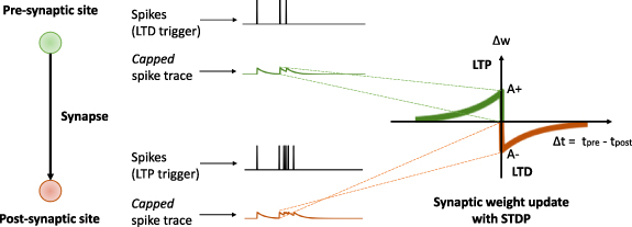
Figure 7. RDSP circuit with highlighted the CMOS building blocks used: eligibility traces (in green), weight updates (in violet) and comparators with differential pair (in yellow). Adapted from [98].
Download figure:
Standard image High-resolution image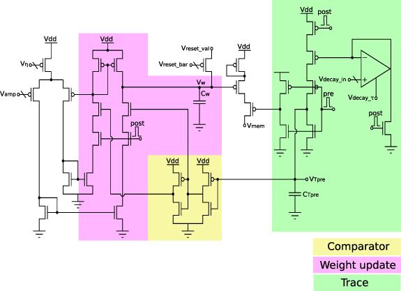
The voltage  is constantly compared to the threshold voltage (resembling
  ) of the first inverter it is connected to. At the arrival of a postsynaptic spike (post is high) the weight capacitor Cw
is either charged (depressed) or discharged (potentiated) depending on the momentary level of
) of the first inverter it is connected to. At the arrival of a postsynaptic spike (post is high) the weight capacitor Cw
is either charged (depressed) or discharged (potentiated) depending on the momentary level of  . If
. If  is above the inverter threshold voltage, the right branch of the weight update block (see figure 7) is inactive, while the left branch is active and the pMOS-based current mirror charges the capacitor Cw
. In the opposite case, where
is above the inverter threshold voltage, the right branch of the weight update block (see figure 7) is inactive, while the left branch is active and the pMOS-based current mirror charges the capacitor Cw
. In the opposite case, where  is below the inverter threshold voltage, the right branch is active while the output of the second inverter disables the left branch of the weight update block. This results in a discharge of the capacitor Cw
controlled by the nMOS-based current mirror. The amplitude for potentiation and depression is set by the two biases Vη
and
is below the inverter threshold voltage, the right branch is active while the output of the second inverter disables the left branch of the weight update block. This results in a discharge of the capacitor Cw
controlled by the nMOS-based current mirror. The amplitude for potentiation and depression is set by the two biases Vη
and  . At the end of a postsynaptic spike the correlation signal
  is reset to Vdd. A similar approach implementing a nearest-spike interaction scheme and a fixed
  was implemented by Ramakrishnan et al [99] exploiting the properties of floating gates.
4.6. Additional models
In this work we covered a large fraction of (if not all) the spike-based learning models implemented using analog neuromorphic electronic circuits presented in the literature to date. The overview and comparison of the theoretical models should therefore enable the implementation of additional models using the principles and circuits presented. For example, novel models that require to keep track of pre- or postsynaptic spiking activity for extended periods of time could make use of circuits such as those described for the SDSP and C-STDP models. Models that require both postsynaptic traces (for potentiation and depression) and a presynaptic trace (for potentiation) could employ the circuits used to describe the V-STDP rule. In general, slowly decaying traces can be implemented with the DPI block present in many of the learning circuits described. To compare signals (e.g. to determine the sign of an error signal), one could use the WTA current mode circuit, used in the SDSP model. To increase or decrease synaptic weight values, one could use the weight update block presented in figure 3, which makes use of a capacitor. To store the value of the learned weight, one would need to digitize and memorize the voltage across the weight capacitance (e.g. using four bits, which have been shown to be sufficient for a wide variety of problems [102]).
Therefore, to implement local spike-based learning models not covered in this survey, one could re-use many of the circuits presented here. However, additional innovation and design efforts might be required for more elaborate learning rules. For instance, the DPSS learning rule requires a multi-compartment neuron circuit, while the the H-MPDP and C-MPDP rules require conductance-based neuron and synapse circuits. Similarly, although the V-STDP rule [46, 63] shares similarities with the T-STDP one, and the main building blocks introduced in the previous section can be used to implement it with analog CMOS neuromorphic circuits, its complexity comes from its multiple transient signals on different timescales. To this end, emerging novel technologies, such as memristors [103â107] and neuristors [108] offer promising solutions to implement different timescales in a compact and efficient manner. Also implementations for the DPSS rule [68] are difficult to implement due to the increased complexity of the required multi-compartment neuron models. Recently, implementations based on hybrid memristorâCMOS systems [109, 110] or using existing neuromorphic processors to exploit neuron structures to replicate the multi-compartment model [111, 112] have been proposed.
5. Discussion and conclusion
5.1. Toward a unified synaptic plasticity framework
In this survey, we highlighted the similarities and differences of representative models of synaptic plasticity and provided examples of neuromorphic CMOS circuits that can be used to implement their principles of computation. We highlighted how the principle of locality in learning and neural computation in general is essential and enables the development of fast, efficient and scalable neuromorphic processing systems. We highlighted how the different features of the plasticity models can be summarized in (1) synaptic weights properties, (2) plasticity update triggers and (3) local variables that can be exploited to modify the synaptic weight (see also table 14). Although all local variables of these rules are similar in nature, the plasticity rules can be subdivided as follows:
- Presynaptic spike trace: RDSP.
- Pre- and postsynaptic spike traces: STDP, T-STDP, C-STDP, SBCM, BDSP.
- Presynaptic spike trace + postsynaptic membrane voltage: V-STDP, DPSS, MPDP, H-MPDP.
- Postsynaptic membrane voltage + postsynaptic spike trace: SDSP, C-MPDP.
Many possibilities arise when exploring how the local variables used by these rules interact (e.g. comparison, addition, multiplication, etc). The heterogeneity of the rules reviewed in this work arises by the dual nature of bottom-up approaches (e.g. driven by biological experiments to assess the spike-time or spike-frequency dependence in learning) and top-down approaches driven by theoretical requirements for solving specific problems (e.g. local approximation of the credit assignment problem in BDSP).
It is difficult to predict whether a unified rule of synaptic plasticity can be formulated, based on the observation that several plasticity mechanisms coexist in the brain [5], and that different problems may require different plasticity mechanisms. However, we provided here a single unified framework that allowed us to systematically overview the features of many representative models of synaptic plasticity developed following experiment-driven bottom-up approaches and/or application-driven top-down approaches [113].
5.2. Overcoming BP limits for online learning
Local synaptic plasticity in neuromorphic circuits offers a promising solution for online learning in embedded systems. However, due to the very local nature of this approach, there is no direct way of implementing global learning rules in multi-layer neural networks, such as the gradient-based BP algorithm [114, 115]. This algorithm has been the work horse of artificial neural networks training in deep learning over the last decade. Gradient-based learning has recently been applied for offline training of SNNs, where the BP algorithm coupled with surrogate gradients is used to solve two critical problems: first, the temporal credit assignment problem which arises due to the temporal inter-dependencies of the SNN activity. It is solved offline with BP through time (BPTT) by unrolling the SNN like standard recurrent neural networks [13]. Second, the spatial credit assignment problem, where the credit or 'blame' with respect to the objective function is assigned to each neuron across the layers. However, BPTT is not biologically plausible [116, 117] and not practical for on-chip and online learning due to the non-local learning paradigm. On one hand, BPTT is not local in time as it requires keeping all the network activities for the duration of the trial. On the other hand, BPTT is not local in space as it requires information to be transferred across multiple layers. Indeed, synaptic weights can only be updated after complete forward propagation, loss evaluation, and BP of error signals, which lead to the so-called 'locking effect' [118]. Furthermore, software implementations of BP and of spike-based learning rules in general, often use learning-rate optimizers such as Adam [119], which requires additional synaptic traces and memory resources which would significantly increase the hardware cost of the plasticity circuits.
Recently, intensive research in neuromorphic computing has been dedicated to bridge the gap between BP and local synaptic plasticity rules [12, 120] by reducing the non-local information requirements, at a cost of accuracy in complex problems [12]. Relaxing BP constraints for neuromorphic hardware often results in three-factor learning rules, where the temporal credit assignment can be handled using eligibility traces [121, 122] that can, for example, solve the distal reward problem by bridging the delay between the network output and the feedback signal that may arrive later in time [123]. Similarly, inspired by recent progress in deep learning, several strategies have been explored to solve the spatial credit assignment problem in three-factor learning rules using feedback alignment [124], direct feedback alignment [125, 126], random error BP [127] or by replacing the backward pass with an additional forward pass whose input is modulated with error information [128â130]. However, these approaches only partially solve the problem [12], since they still suffer from the locking effect, which can nevertheless be tackled by replacing the global loss by a number of local loss functions [13, 131â133] or by using direct random target projection [113, 134]. The assignment of credit locally, especially within recurrent SNNs, is still an open question and an active field of research [135].
The local synaptic plasticity models and circuits presented in this survey do not require the presence of a teacher signal in the form of a third factor and contrast with supervised learning using labeled data which is neither biologically plausible [133] nor practical in most online scenarios [136]. Nevertheless, the main limit of spike-based local learning is the diminished performance on complex pattern recognition problems. Different approaches have been explored to bridge this gap, for example using multi-compartment neurons to approximate BP with local mechanisms as in the DPSS [68, 69] and BDSP [44] learning rules, developing global gradient-based approaches to train offline the local plasticity mechanisms that will be used online [137â140], or exploring multimodal association to improve the self-organizing system's performance [20, 21, 141] since in contrast to labeled data, multiple sensory modalities (e.g. sight, sound, touch) are freely available in the real-world environment.
5.3. Challenges of three-factor local plasticity
In three-factor learning rules, in addition to depending on state-variables present at the pre- and postsynaptic terminals, the weight update depends also on a third signal, which can come from a phasic increase of neuromodulators such as dopamine and serotonin, or from an additional spiking input [26]. From a top-down approach, these types of learning rules have been used to approximate the BP learning algorithm, and have been used to solve practical real-world problems with very promising results (e.g. see the e-prop rule [122], the deep continuous local learning (DECOLLE) rule [132], or the event-based three-factor local plasticity (ETLP) rule [134]). From a bottom-up approach, these types of rules can be implemented using biologically plausible mechanisms and signals in neuromorphic hardware. However the extra flexibility and computational power offered by these rules comes at a cost of additional resources. For example, many of these rules require additional synaptic traces or eligibility traces with very long decay rates (e.g. at behavioral time scales of seconds to minutes). This would require circuits with very long time constants at each synapse, achievable with either very large capacitors or very large resistors or both. This would in turn require large area overhead (e.g. in case of large capacitors for each synapse), or large power consumption (e.g. in case of having to operate circuits with very large impedance values). In addition, the signals that represent the third factor are typically non-local, and require dedicated means of transmission (e.g. via broadcast routing schemes, or global bias values that need to be modulated hardwired in need to be broadcast to large populations). These limitations and challenges need to be addressed both at the algorithmic level and at the hardware level, following a tightly integrated co-design approach, that has only been used in rare cases so far [113].
5.4. Structural plasticity and network topology
Exploring local synaptic plasticity rules could provide valuable information on how plasticity results in learning and memory in the brain. However, in bringing the plasticity of single synapses to the function of entire networks, many more factors come into play. Functionality at a network level is determined by the interplay between the synaptic learning rules, the spatial location of the synapse, and the neural network topology. Furthermore, the brain network topology is itself plastic [142]. Le Bé and Markram [143] provided the first direct demonstration of induced rewiring (i.e. sprouting and pruning) of a functional circuit in the neocortex [144], which requires hours of general stimulation. Some studies suggest that glutamate release is a key determinant in synapse formation [145, 146], but additional investigations are needed to better understand the computational foundations of structural plasticity and how it is linked to the synaptic plasticity models we reviewed in this survey. Together, structural and synaptic plasticity are the local mechanisms that lead to the emergence of the global structure and function of the brain. Understanding, modeling, and implementing the interplay between these two forms of plasticity is a key challenge for the design of self-organizing systems that can come closer to the unique efficiency and adaptation capabilities of the brain.
5.5. CMOS neuromorphic circuits
The computational primitives that are shared by the different plasticity models were grouped together in corresponding functional primitives and circuit blocks that can be combined to map multiple plasticity models into corresponding spike-based learning circuits. Many of the models considered rely on exponentially decaying traces. By operating the CMOS circuits in the sub-threshold regime, this exponential dependency is given by the physical substrate of transistors showing an exponential relationship between current and voltage [10, 147].
The circuits presented make use of both analog computation (e.g. analog weight updates) and digital communication (e.g. pre- and postsynaptic spike events). This mixed-signal analog/digital approach aligns with the observations that biological neural systems can be considered as hybrid analog and digital processing systems [148]. Due to the digital nature of spike transmission in these neuromorphic systems, plasticity circuits that require the use of presynaptic traces need extra overhead to generate this information directly at the postsynaptic side. The emergence of novel nanoscale memristive devices has high potential for allowing the implementation of such circuits at a low overhead cost, in terms of space and power [149]. In addition, these emerging memory technologies have the potential of allowing long-term storage of the synaptic weights in a non-volatile way, that would allow these neuromorphic systems to operate continuously, without having to upload the neural network parameters at boot time. This will be a significant advantage in large-scale systems, as input/output operations required to load network parameters can take a significant amount of power and time. In addition, the properties of emerging memristive devices could be exploited to implement different features of the plasticity models proposed [107].
Overall, the number of proposed CMOS-based analog or mixed-signal neuromorphic circuits over the past 25âyears was mainly driven by fundamental academic research taking place is a handful laboratories. However, with the increasing need for low-power neural processing systems at the edge, the increasing maturity of novel technologies, and the rising interest in brain-inspired neural networks and learning for data processing, we can expect an increasing number of new mixed signal analog/digital circuits implementing new plasticity rules also for commercial exploitation. In this sense, this review can provide valuable information to make informed decisions about circuit design and modeling in developing novel spike-based neuromorphic processing systems for online learning.
Acknowledgments
We would like to thank the BICS group at the University of Groningen, and the NCS group at the Institute of Neuroinformatics of the University of Zurich and ETH Zurich for fruitful discussions. We would also like to thank Hugh Greatorex, Maxime Fabre, Jannes Jegminat, Samuel R Schmidgall, Ali Safa, Sebastian Schmitt, Adam Kohan and Carver Mead for providing valuable feedback on the first revisions of the manuscript, Madison Cotteret for the helpful comments on the equations details and Michele Mastella and Wouter Serdijn for the fruitful discussions on circuit details. We want to acknowledge the financial support of the CogniGron research center and the Ubbo Emmius Funds (University of Groningen), the European Union's H2020 research and innovation programme under the H2020 'BeFerroSynaptic' Project (No. 871737), the MSCA ITN 'MANIC' Project (No. 861153), the EU ERC 'NeuroAgents' Project (No. 724295), the Swiss National Science Foundation 'Sinergia' Project (CRSII5-18O316).
Data availability statement
No new data were created or analyzed in this study.
Supplementary material (0.1 MB PDF) A historical, experimental and theoretical perspectives on synaptic plasticity.