Structured robust correlation filter with L2,1 norm for object tracking

Yongjin Guo; Shunli Zhang; Feng Bao

doi:10.1117/1.JEI.28.6.063005

20 November 2019 Structured robust correlation filter with L_2,1 norm for object tracking

Yongjin Guo, Shunli Zhang, Feng Bao

Author Affiliations +

Journal of Electronic Imaging, Vol. 28, Issue 6, 063005 (November 2019). https://doi.org/10.1117/1.JEI.28.6.063005

Abstract

Recently, the correlation filter (CF)-based methods have achieved great success in the field of object tracking. In most of these methods, the CF utilizes L₂ norm as the regularization, which does not pay attention to the stability and robustness of the feature. However, there may exist some unstable points in the image because the object in the video may have different appearance changes. We propose a tracking method based on a structured robust correlation filter (SRCF), which employs the L_2,1 norm as the regularization. The robust CF can not only retain the accuracy from the regression formulation but also take into account the stability of the image region to improve the robustness of the appearance model. The alternating direction method of multipliers algorithm is used to solve the L_2,1 optimization problem in SRCF. Moreover, the multilayer convolutional features are adopted to further improve the representation accuracy. The proposed method is evaluated in several benchmark datasets, and the results demonstrate that it can achieve comparable performance with respect to the state-of-the-art tracking methods.

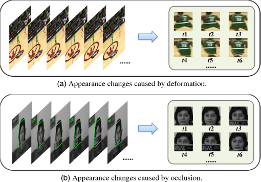
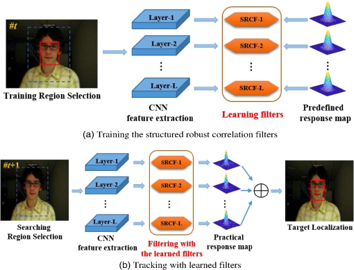
1. Introduction

Visual object tracking is a hot research topic in the domains of computer vision, multimedia, etc. It has been successfully used in many fields, such as video surveillance,¹^,² traffic monitoring,³ and motion analysis, and has attracted the attention of more researchers.⁴^,⁵ However, realizing accurate and robust tracking is still a challenging task because there are many complex conditions, including appearance deformation, occlusion of similar or different objects, illumination variations, scale changes, background clutter, etc.

According to the appearance model, the tracking methods can be divided into two types, i.e., the generative model⁶^–¹² and the discriminative model.¹³^–¹⁷ The generative model often formulates tracking as a matching problem, which only uses the information of the target. On the contrary, the discriminative model utilizes the information of both the target and the background, which is always formulated as a binary classification or a regression problem. Because the discriminative model-based methods use more information, they can get better performance during the tracking process. Furthermore, the regression formulation, which uses more spatial information, attracts more attention because it replaces the sparse sampling in binary classification with dense sampling.

Recently, some tracking methods based on a correlation filter (CF), which corresponds to the regression formulation, have achieved great success.¹⁸^–²¹ On one hand, the CF addresses the sparse sampling in binary classification model, which makes full use of the spatial information. On the other hand, by introducing circulant assumption to generate training samples, CF can greatly improve the efficiency of sample selection and speed up the training and detection process by fast Fourier transform (FFT). Bolme et al.¹⁸ first model the appearance by learning the CF and propose a minimum output sum-of-squared error filter tracking method, but this method does not make full use of the spatial constraints. Henriques et al.¹⁹^,²² exploit the circulant structure of the local image patch and learn a ridge regression as well as a CF for tracking. Danelljan et al.²³ develop the adaptive color attributes based tracker by adding the color attribute to augment the intensity feature. Zhang et al.²⁴ incorporate geometric transformations into a CF-based network to handle boundary effect issue.

Inspired by the successful applications in face recognition, image detection, image classification, etc., deep learning has been introduced into tracking by some researchers as well. For example, Wang and Yeung²⁵ introduce an autoencoder into tracking and develop the first deep learning-based tracker. Li et al.²⁶ present a single convolutional neural network (CNN) based tracking method, which can learn effective feature representations. Nam and Han²⁷ propose to learn multidomain CNN for tracking, which is composed of shared layers and multiple branches of domain-specific layers. Due to the powerful representation ability, deep learning greatly improves the tracking performance. Commonly, deep learning works together with the generative model, different classifiers, or regression algorithms, thus, the tracking methods with deep learning still retain the disadvantages of these formulations.

Recently, some researchers²⁸^–³¹ have also proposed some new tracking methods, which utilize both the deep CNN and CF to further improve the tracking performance. For example, Ma et al.²⁸ develop the hierarchical convolutional features based tracking, which exploits the multiple levels of abstraction for pyramid representation under the CF tracking framework. Mueller et al.³⁰ present the context-aware CF tracking, which takes global context into account and incorporates it into the CF. Danalljan et al.²⁹ introduce a factorized convolution operation and a compact generative model of the training sample distribution in CF tracking, which greatly improves the tracking efficiency. However, in most of these methods, only $L_{2}$ norm is used and less attention is focused on the unstable positions in the image region. In practice, because of the appearance changes caused by deformation or occlusion (Fig. 1), there always exist unstable points in the region.

Fig. 1

Appearance changes caused by (a) deformation and (b) occlusion.

In this study, we propose a tracking method based on the structured robust correlation filter (SRCF) with $L_{2,1}$ norm. First, to address the impact of the unreliable points in the image region with a multichannel feature, we develop a robust CF and formulate tracking as a structured robust regression problem. By introducing the structured sparse formulation, the stable features can be adaptively selected. Further, we derive the solution algorithm corresponding to the SRCF based on alternating direction method of multiplier (ADMM) approach. Second, based on the traditional CF tracking methods, we implement a concrete tracking algorithm based on the proposed SRCF. Specifically, we extract the multilayer multichannel features with CNN for representation, which can further improve the representation ability. Moreover, we also present a judgment-based update model to improve the tracking robustness in complex conditions. We evaluate the performance of the proposed tracking methods on many public datasets, and the experimental results illustrate that the proposed tracking method based on SRCF with $L_{2,1}$ norm can achieve comparable performance to many state-of-the-art trackers.

The remainder of this study is organized as follows. In Sec. 2, we introduce the related work of classical CF-based tracking. In Secs. 3 and 3.5, we describe the proposed SRCF and its corresponding tracking method, respectively. Section 4 shows the experimental results and the last section concludes the study.

2. Correlation Filter Tracking

Before discussing our proposed tracking method based on the robust CF, we first review the tracking method based on the traditional CF.²² Hereby, we briefly introduce the key components of the CF tracker, which includes the ridge regression formulation, fast realization with FFT, the dense sampling, and the circulant assumption.

The CF corresponding to the ridge regression is represented as follows:

Eq. (1)

\min_{w} λ {‖ w ‖}_{2}^{2} + {‖ Xw - y ‖}_{2}^{2},

where

w

denotes the model parameter,

X = {[x_{(1)}, x_{(2)}, \dots, x_{(n)}]}^{T}

,

x_{(i)}

denotes a training sample,

y = {[y_{1}, y_{2}, \dots, y_{n}]}^{T}

, and

y_{i}

is the label corresponding to

x_{(i)}

.

Based on the circulant assumption, we can obtain the solution to 1 in Fourier domain:

Eq. (2)

\hat{w} = \frac{{\hat{x}}^{*} ⊙ \hat{y}}{{\hat{x}}^{*} ⊙ \hat{x} + λ},

where

\hat{w}

and

\hat{x}

corresponding to the Fourier transform of

w

and

x

, respectively,

⊙

denotes the elementwise multiplication, and

\hat{y}

is the Fourier transform of

y

. With the learned

\hat{w}

, the filtering response

r

can be obtained in the following frame.

CF tracking brings many benefits. First, by formulating tracking as a regression problem, the spatial information of the image can be fully utilized, and the appearance model built based on the CF can be represented more accurately. Second, based on the circulant assumption, much more training samples can be generated virtually without increasing the computation complexity. Since the regularization term in the traditional filter is $L_{2}$ norm, it can be realized fast by using FFT algorithm. However, because the object is always moving in the video sequences, the appearance of the object may change heavily, which will generate unstable regions. In this condition, $L_{2}$ norm is not robust to the outlier points and the appearance model may be not accurate enough.

3. Tracking with Structured Robust Correlation Filter

3.1.

Overview

To address the unstable points and improve the accuracy of the appearance model, we formulate tracking as a robust regression problem and develop a SRCF-based tracking method. The overview of the proposed method is shown in Fig. 2. Different from the traditional ridge regression formulation, we formulate tracking as a structured robust regression problem with $L_{2,1}$ norm, which can adaptively select the robust features for tracking. First, the SRCF with $L_{2,1}$ norm regularization, which is built based on the training region and predefined response map, is trained. Then, the learned filter is used for tracking in the following frame. Specifically, the multilayer CNN features are used to improve the representation ability. Moreover, an update model with judgment and incremental strategies is constructed to accommodate the filters.

Fig. 2

Overview of the proposed tracking method: (a) Training the SRCFs and (b) tracking with learned filters.

3.2.

$L_{1}$ Norm Based Robust Correlation Filter

We first introduce the robust CF with $L_{1}$ norm, which is suitable for the single-channel feature. In this condition, each element of the feature corresponds to a specific position in the image region. Therefore, using $L_{1}$ norm can adaptively choose the stable points, alleviating the effect of the appearance changes.

Assume that the training sample matrix is denoted as $X$ , whose element is $x_{(i)}$ and its corresponding label is denoted as $y_{i}$ . Similar to the sample generation in the traditional CF, $X$ can be approximately obtained by circular shifts of $x$ . Inspired by the feature selection property of the $L_{1}$ norm and considering the stability of the points, we develop the CF with $L_{1}$ norm:

Eq. (3)

\min_{w} λ {‖ w ‖}_{1} + {‖ Xw - y ‖}_{2}^{2} .

Note that

L_{1}

norm is used as the regularization term to replace the original

L_{2}

norm.

3.3.

$L_{2,1}$ Norm-Based Structured Robust Correlation Filter

$L_{1}$ norm is only suitable for the single-channel feature. Since the single-channel feature always means intensity, it is not able to represent the appearance accurately. Commonly, to improve the representation ability, the single-channel feature can be extended to multichannel feature, such as histogram of oriented gradient (HOG), CNN, etc. In the condition of multichannel feature, there is a group of feature elements in each specific position of the image region. Choosing the specific group of features can be taken as a structured sparse learning problem, which can be solved by $L_{2,1}$ norm. Thus, $L_{1}$ norm is extended to $L_{2,1}$ norm to select the stable feature group. Correspondingly, the new CF with $L_{2,1}$ norm regularization is named SRCF.

The CF with $L_{2,1}$ norm regularization can be represented as

Eq. (4)

\min_{W} {‖ Σ_{j} X_{j} W_{j} - y ‖}_{2}^{2} + λ {‖ W ‖}_{2,1},

where

W

denotes the multichannel parameter,

W_{j}

means the

j

’th channel of

W

, and

X_{j}

is the

j

’th channel of

X

.

3.4.

Optimization

We employ the ADMM algorithm to solve the problem in Eq. (4). By introducing the auxiliary variable $V$ and adding more constraints, Eq. (4) becomes

Eq. (5)

\min_{W} {‖ Σ_{j} X_{j} W_{j} - y ‖}_{2}^{2} + λ {‖ V ‖}_{2,1},

which is subject to

V = W .

Then, the Lagrange function can be represented as

Eq. (6)

L = {‖ Σ_{j} X_{j} W_{j} - y ‖}_{2}^{2} + λ {‖ V ‖}_{2,1} + ⟨ U, V - W ⟩ + \frac{ρ}{2} {‖ V - W ‖}_{F}^{2},

where

U

is the Lagrange multiplier and

ρ

is the penalty parameter. The parameters can be iteratively updated under ADMM framework. The detailed solving process is explained as follows.

First, update $W$ with the other parameters fixed. In this condition, the optimization problem becomes

Eq. (7)

\min_{W} {‖ Σ_{j} X_{j} W_{j} - y ‖}_{2}^{2} + ⟨ U, V - W ⟩ + \frac{ρ}{2} {‖ V - W ‖}_{F}^{2} .

By setting the gradient of Eq. (7) with respect to $W$ to 0, we can get the closed-form solution:

Eq. (8)

W_{j} = Σ_{k} {(X_{k}^{T} X_{k} + ρ I)}^{- 1} (X_{j}^{T} y + ρ V_{j} + U_{j}),

where

V_{j}

and

U_{j}

denote the

j

’th channel of

V

and

U

, respectively.

Based on the circulant assumption, the feature matrix $X_{j}$ can be obtained by circular shifts of $x_{j}$ , where $x_{j}$ is the $j$ ’th channel of the center sample feature map $x$ . Thus, by FFT algorithm, the Fourier transform of the parameter $W$ in the $j$ ’th channel is represented as follows:

Eq. (9)

{\hat{W}}_{j} = \frac{{\hat{x}}_{j}^{*} ⊙ \hat{y} + ρ {\hat{V}}_{j} + {\hat{U}}_{j}}{Σ_{k} {\hat{x}}_{k}^{*} ⊙ {\hat{x}}_{k} + ρ} .

Second, update $V$ with the other parameters fixed. Hereby, the optimization problem becomes

Eq. (10)

\min_{V} λ {‖ V ‖}_{2,1} + \frac{ρ}{2} {‖ V - W + U / ρ ‖}_{2}^{2} .

The problem with both $L_{2,1}$ norm and $L_{2}$ norm in Eq. (10) has a closed-form solution:

Eq. (11)

V = \max (0,1 - \frac{λ}{ρ {‖ W - U / ρ ‖}_{2}}) (W - U / ρ) .

Third, the rest of the parameters can be updated as follows:

Eq. (12)

U \leftarrow U + ρ (V - W) ρ \leftarrow μ ρ,

where

μ

is the update coefficient. By iteratively updating

W

,

V

,

Z

, and

μ

for several times, the solution can be convergent. Then, the model can be built and used for tracking in the following frames.

3.5.

Tracking with SRCF

Under the CF tracking framework, we develop the tracking method with the proposed SRCF. Moreover, we utilize the convolutional feature to represent the appearance and use a judgment strategy to improve the accuracy of the update model.

3.5.1.

Representation

The representation in tracking includes two parts: selection of the training and searching regions and feature extraction. Since we follow the CF tracking framework, we adopt the same region selection scheme. For the training region, we select an image region that has the same center as the target and a much larger area. On one hand, the larger region can satisfy the circulant assumption, which is useful for the fast realization with FFT. On the other hand, because the training samples are sampled approximately based on circular shifts, the larger region indicates the dense sampling, which improves the discriminability of the model. The searching region is selected in the next frame according to the same manner as the training region.

Once the training or searching region is selected, specific features can be extracted for better representation. In the original CF tracking method and some variants, both the intensity and HOG features are adopted. Inspired by the powerful representation ability of convolutional features, we extract the convolutional features via VGG-Net, which is trained in the ImageNet dataset and achieves excellent performance on classification and detection challenges. Different layers of the features describe the image from different aspects, i.e., the lower layers have more location information while the higher layers keep more semantic information. Because both location and semantic information is important for tracking, we use several layers of the convolutional features for representation.

3.5.2.

Training SRCF

Because the convolutional features with multiple layers are used for representation, we train a multilayer SRCF group as the appearance model. Assume that the feature map of the training region in the $l$ ’th layer is $X^{l}$ . According to Eqs. (7)–(12), we can train an individual SRCF corresponding to each feature layer. Then, the CFs in all layers are collected and taken as the model ${{\hat{W}}^{l}}$ for tracking.

3.5.3.

Determining the tracking result

Assume the multichannel feature map of the searching region in the $l$ ’th layer is $Z^{l}$ . Based on the trained SRCF ${W^{l}}$ and its Fourier transform ${{\hat{W}}^{l}}$ , we can calculate the response map $\hat{r}$ in the Fourier domain:

Eq. (13)

\hat{r} = Σ_{l} w_{l} Σ_{j} {\hat{W}}_{j}^{l} ⊙ {\hat{Z}}_{j}^{l},

where

{\hat{Z}}_{j}^{l}

is the

j

’th channel of

{\hat{Z}}^{l}

and

w_{l}

denotes the weight of the

l

’th layer. By calculating the IFFT of

\hat{r}

, we can get the response map

r

in the spatial domain. Further, the final tracking result is determined by the maximum of

r

.

3.5.4.

Model update

To better capture the changes of the appearance, the CF should be updated in a timely manner. Besides, online learning should be adaptively controlled to avoid learning the occlusion. In our method, the model update includes two stages. In the first stage, to alleviate the impact of the occlusion, we present a judgment strategy to control the update. We calculate the cosine similarity of two consecutive frames:

Eq. (14)

s (x_{I}^{t}, x_{I}^{t - 1}) = \frac{x_{I}^{t T} x_{I}^{t - 1}}{{‖ x_{I}^{t} ‖}_{2} {‖ x_{I}^{t - 1} ‖}_{2}},

where

x_{I}^{t}

denotes the intensity feature of the region in

t

’th frame. If

s (x_{I}^{t}, x_{I}^{t - 1})

is larger than a predefined threshold

T h_{u}

, it is considered that the current model can retain the accuracy and we do not update model. Otherwise, the model needs to be updated to capture the changes of the appearance model. By the judgment strategy, the over learning of the occlusion can be alleviated while the significant changes can be learned timely.

In the second stage, we utilize an incremental strategy to realize the model update. Once it is determined to update, we can select a new training region in the current frame and extract its multichannel feature. Then, the model is updated by

Eq. (15)

A^{l} (t) = θ A^{l} (t - 1) + (1 - θ) {\hat{X}}^{l} (t), B^{l} (t) = θ B^{l} (t - 1) + (1 - θ) {\hat{X}}^{l *} (t) ⊙ {\hat{X}}^{l} (t),

where

X^{t}

is the feature map extracted from the current frame,

A (t)

and

B (t)

denote the molecular and denominator for training in the current frame,

A (1) = X (1)

,

B (1) = {\hat{X}}^{*} (1) ⊙ \hat{X} (1)

, and

θ

denotes the update rate. Then, by iteratively solving the problems in Eqs. (7) and (10), the new tracking model can be trained with

A^{t}

and

B^{t}

.

3.5.5.

Scale adaption

During the tracking process, the scale of the object may be changed. To obtain better tracking performance, we adopt the scale adaption strategy²³ to address the scale changes. Besides the translation filters used for location, the scale filter is built to estimate the optimal scales of the target. The scale filter is learned based on the image patch centered around the target and 33 scales are used for scale estimation (Algorithm 1).

Algorithm 1

SRCF tracking: iteration in frame t.

Input:

Frame

I_{t}

; Previous object position

p_{t - 1}

; Robust filter

{W^{l}}

.

Output:

Object position

p_{t}

and corresponding bounding box; Updated filter

{W^{l}}

.

1: Tracking.

(1) Crop the candidate image patch at

p_{t - 1}

from

I_{t}

and extract the convolutional features conv3-4, conv4-4 and conv5-4 of VGG-Net-19;

(2) Calculate the response map

\hat{r}

by Eq. (13);

(3) Determine the optimal position

p_{t}

by taking the maximum value of

\hat{r}

.

2: Update.

(1) Crop the training patch at

p_{t}

from

I_{t}

, and extract and augment the features conv3-4, conv4-4 and conv5-4 of VGG-Net-19;

(2) Judge whether to update by calculating the similarity

s

with Eq. (14).

IF:

s > T h_{s}

, NOT update;

ELSE:

(2.1) Update the

A^{l} (t)

and

B^{l} (t)

by Eq. (15);

(2.2) Learn the filter

{W^{l}}

by solving Eq. (4) with ADMM.

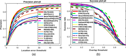
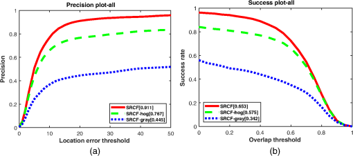
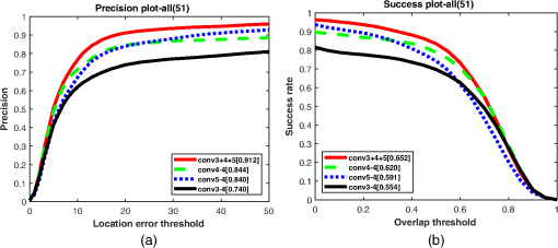
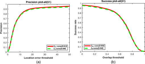
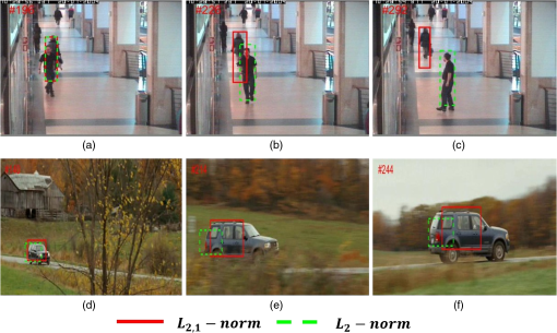
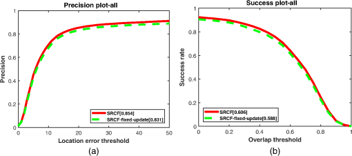
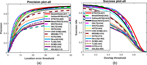
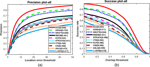
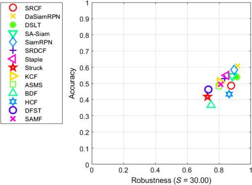
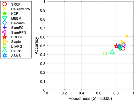
4. Experiments

4.1.

Implementation Details

We denote the proposed tracking method as SRCF, which is initialized as follows. VGG-Net-19 network is used to extract features and the outputs of the conv3-4, conv4-4 and conv5-4 are taken as the features. For each layer of the feature, we train a corresponding model and the final tracking response map is the summation of the response in the above three layers. The weights of the above three layers are set as 1, 0.5, and 0.25, respectively. For the Gaussian function, $σ^{2} = 0.1$ . The regularization parameter $α$ is set as 0.01. The coefficient $ρ$ is set as 3 and the iterations for ADMM are set as 15. The judging threshold is set as 0.99 and the update rate is set as 0.99. The padding factor for the larger region selection is set at 1.8. All parameters are fixed for all sequences.

The precision plots and success plots, which are obtained by precision and success rate (SR), are used to evaluate the performance of the trackers. Precision is calculated by the ratio of the number of frames in which center location error is smaller than a threshold $T h_{p}$ and the number of the total frames. Visual overap rate (VOR) is defined as the average of $Score = \frac{area (R_{S} \cap R_{G})}{area (R_{S} \cup R_{G})}$ , where $R_{S}$ and $R_{G}$ represent the bounding boxes of the tracking result and ground truth, respectively.³² SR is defined as the ratio of the number of success frames and the total frames, where tracking in one frame is taken to be successful if the VOR in that frame is larger than a predefined threshold $T h_{s}$ . By assigning different values to $T h_{p}$ and $T h_{s}$ , the precision plots and success plots can be obtained to display the overall performance. The area under the curve (AUC) is used as another evaluation criterion as well.

4.2.

Comparison with State-of-the-Art Methods

We compare the performance of the proposed SRCF tracking method with several state-of-the-art tracking methods in the OTB-2013 dataset.³³ The competing trackers include DSLT,³⁴ MetaCREST,³⁵ MetaSDNet,³⁵ DaSiamRPN,³⁶ STRCF,³⁷ CNNSVM,³⁸ MEEM,³⁹ KCF,²² Struck,⁴⁰ SCM,⁴¹ TLD,⁴² ASLA,⁴³ HDT,⁴⁴ and CXT.⁴⁵

We first evaluate the overall performance of the proposed SRCF tracker and the competing trackers. The comparison results are shown in Fig. 3, which displays the precision plots and the success plots of SRCF and the competing trackers. It can be seen that our SRCF achieves the precision at 20 pixels 0.911, which ranks the second among the trackers, and obtains the AUC score 0.653, which ranks the fifth and outperforms most of the competing trackers.

Fig. 3

(a) Precision plots and (b) success plots of SRCF and the competing trackers on all 51 sequences in OTB-2013. The precision at $T h_{p} = 20 pixels$ and the AUC score are put in the bracket behind the name of the tracker.

4.3.

Ablation Study

4.3.1.

Feature representation

In our method, we exploit the powerful representation ability of the CNN and extract the features from three different layers of VGG-Net-19 for representation. To verify the role of the CNN features, we build another two trackers, which only use the handcrafted features, i.e., HOG and grayscale features for comparison. We evaluate the performance of the trackers in the OTB-2013 dataset and show the result in Fig. 4. It can be found that the tracker with CNN feature achieves better performance on both the precision and success plots. Specifically, we can also see that the precision at 20 pixels and AUC obtained by the SRCF tracker with only HOG feature also outperform the KCF method by 2.5% and 5.9%, respectively.

Fig. 4

(a) Precision plots and (b) success plots of the trackers with different features.

Since we use three different layers of VGG-Net-19, i.e., the conv3-4, conv4-4, and conv5-4 for comprehensive representation, we further implore the contribution of each layer. Besides the standard tracker, which uses all of the three layers, we build another three trackers, each of which makes use of the feature in a single layer. The comparison results on OTB-2013 are shown in Fig. 5. It can be seen that, among the competing trackers, the tracker with the conv4-4 obtains the best precision and success plots, the tracker with the conv5-4 achieves the second-best results, and the tracker with the conv3-4 ranks the third. However, by combing features in all of the three layers, the tracking performance can be further improved, indicating that all three layers have a significant contribution for tracking.

Fig. 5

(a) Precision plots and (b) success plots of the trackers with different layers.

4.3.2.

Analysis of regularization

The main difference between our formulation and the traditional tracking methods is that we adopt the structured robust regularization with $L_{2,1}$ norm instead of the original $L_{2}$ norm (Frobenius norm for multichannel feature). Hereby, we explore the contribution of $L_{2,1}$ norm by building a new comparison tracker with $L_{2}$ norm. Hereby, the CF with $L_{2}$ norm has the same configuration with the standard SRCF except the norm regularization.

The comparison results on the OTB-2013 dataset are shown in Fig. 6. It can be found that the precision at $T h_{p} = 20 pixels$ of the tracker with $L_{2,1}$ norm is 0.912, whereas the precision obtained by the $L_{2}$ norm is 0.898. The AUC score of $L_{2,1}$ norm is 0.652, which outperforms the $L_{2}$ norm by 1%. Figure 7 shows two examples that SRCF with $L_{2,1}$ norm gets better results than CF with $L_{2}$ norm. Note that the proposed SRCF outperforms the traditional CF tracking method, indicating that the $L_{2,1}$ norm achieves better robustness than the $L_{2}$ norm.

Fig. 6

(a) Precision plots and (b) success plots of SRCF with $L_{2,1}$ norm and the CF with $L_{2}$ norm in OTB-2013.

Fig. 7

Examples of the SRCF with $L_{2,1}$ norm and the CF with $L_{2}$ norm. (a)–(c) Sequence walking2 and (d)–(f) carscale.

4.3.3.

Analysis of model update

In our method, we develop a judgment-based update model to adaptively learn the appearance changes, which can effectively handle the appearance changes and occlusion problems. To explore the impact of the judgment-based update model, we also build a tracker, which only uses the traditional update model without judgment. The comparison results in OTB-100 dataset are shown in Fig. 8. It can be seen that the precision and AUC score of the SRCF tracker with judgment outperform that without judgment by 2.3% and 1.8%, respectively, indicating that the performance of SRCF can be further improved by introducing the judgment-based update.

Fig. 8

(a) Precision plots and (b) success plots of update with and without judgment.

4.4.

Evaluation in More Datasets

Besides the OTB-2013 dataset in which the SRCF tracker has achieved good results, we also evaluate its performance in more datasets, including the Tcolor128 dataset,⁴⁶ OTB-100 dataset,⁴⁷ VOT2016 dataset,⁴⁸ and VOT2017⁴⁹ dataset to explore the effect of the settings of the tracker.

4.4.1.

Evaluation in the OTB-100 dataset

We further evaluate the performance of SRCF in OTB-100 dataset, which includes 100 different sequences. We compare SRCF with several famous tracking methods, including DSLT,³⁴ MetaCREST,³⁵ MetaSDNet,³⁵ DaSiamRPN,³⁶ STRCF,³⁷ CNNSVM,³⁸ MEEM,³⁹ KCF,²² Struck,⁴⁰ SCM,⁴¹ TLD,⁴² ASLA,⁴³ HDT,⁴⁴ and CXT⁴⁵ in this dataset. The comparison results of precision plots and success plots are shown in Fig. 9. We can see that SRCF achieves similar performance to that in OTB-2013 dataset. The precision at $T h_{p} = 20 pixels$ of SRCF is 0.854, which ranks the fifth among the competing trackers and AUC score is 0.613, which ranks the sixth.

Fig. 9

(a) Precision plots and (b) success plots of SRCF and the competing trackers in OTB-100 dataset.

4.4.2.

Evaluation in the Tcolor128 dataset

There are 128 color sequences in the Tcolor128 dataset, in which the sequences are collected from various circumstances, including highway, airport terminal, railway station, etc. Hereby, we evaluate our SRCF tracker in the Tcolor128 dataset with the competing trackers, which include ECO,²⁹ ADNet,⁵⁰ MEEM,³⁹ KCF,²² Struck,⁴⁰ VTD,⁵¹ CN2,²³ ASLA,⁴³ and L1APG.⁵² The overall precision plots and the success plots over the whole dataset are shown in Fig. 10. It can be observed that the precision at $T h_{p} = 20 pixels$ obtained by SRCF is 0.698, and the AUC score is 0.504, both of which rank the third among the competing trackers. In this dataset, the MEEM method achieves good results on both criteria. Since MEEM adopts the color feature, the encoded LAB color model greatly improves the performance. However, ECO, ADNet, and our SRCF tracker, which use deep convolutional features, have more powerful representation ability and get better tracking performance. Moreover, we would like to encode the color feature to further improve our method as well.

Fig. 10

(a) Precision plots and (b) success plots of SRCF and the competing trackers in Tcolor128 dataset.

4.4.3.

Evaluation in the VOT2016 and VOT2017 datasets

We further evaluate the performance of SRCF in VOT2016 and VOT2017 datasets, each of which contains 60 challenging sequences. The accuracy and robustness scores are used as the criteria for evaluation. In VOT2106 dataset, we mainly compare our method with DaSiamRPN, DSLT, SA-Siam,⁵³ SiamRPN,⁵⁴ SRDCF, Staple,⁵⁵ Struck, KCF, ASMS,⁵⁶ BDF,⁵⁷ HCF,²⁸ DFST,⁵⁸ and SAMF,⁵⁹ and the comparison results are shown in Fig. 11. Our SRCF tracker ranks the eighth on accuracy and fifth on the robustness. We also compare our method with DasiamRPN, KCF, MEEM, SA-Siam, SiamFC, SiamRPN, SRDCF, Staple, L1APG, Struck, and ASMS in VOT2017 and display the results in Fig. 12. It can be seen that the proposed SRCF tracker gets better robustness than most trackers, indicating that the $L_{2,1}$ norm can improve the robustness to some degree.

Fig. 11

Precision plots and success plots of SRCF and the competing trackers in VOT2016 dataset.

Fig. 12

Precision plots and success plots of SRCF and the competing trackers in VOT2017 dataset.

4.5.

Running Speed

The running speed is also important for the tracker. Our method is implemented in MATLAB on a PC with an Intel i7 CPU 3.4 GHz and a Nvidia GTX1080 GPU. We compare the running speed of our SRCF and some famous trackers in OTB-100 dataset and show the result in Fig. 1. We can see that the SRCF runs at $1.55 frames / s$ , which is similar to MDNet,²⁷ LSART,⁶⁰ faster than C-COT,⁶¹ SCM, and slower than KCF, DaSiamRPN, MEEM, DSLT, STRCF, and MetaCREST. Although the $L_{2,1}$ norm increases the robustness, it also decreases the running speed. Thus, some parallel strategies will be explored to further improve the running speed in the future.

Since our SRCF tracker is realized based on the CF tracking framework, it retains many advantages of CF tracking methods. For example, it can make full use of the spatial information of the training region, which can improve the representation accuracy. Moreover, it also borrows the feature extraction method from the deep learning algorithms, which further improves the representation ability. Compared to the methods that also follow the CF tracking methods, e.g., ECO, STRCF, SRDCT, Staple, and HDT, our SRCF tracker runs slower because of the $L_{2,1}$ norm, but it also improves the tracking robustness by adaptively selecting the robust features. On the other hand, compared to the methods that adopt the end-to-end deep neural network, such as SiamRPN, DaSiamPRN, MetaSDnet, and LSART, SRCF may obtain some lower accuracy but does not need complex training process. In addition, compared to the sparse learning-based methods, such as SCM, L1APG, and ASLA and ensemble learning-based methods, such as MEEM, SRCF has significant advantages on both accuracy and robustness (Table 1).

Table 1

The comparison of running speed of SRCF and some famous trackers in the OTB-100.

Methods	KCF	DaSiamRPN	MEEM	ECO	DSLT	STRCF	MetaCREST	MDNet	LSART	C-COT	SCM	SRCF
FPS	172	160	10	17.9	5.7	5.3	3.51	1.7	1.3	0.7	0.37	1.55

5. Conclusion

In this study, we present a tracking method based on SRCF. Different from the traditional CF, which only uses $L_{2}$ norm for regularization, the proposed method introduces $L_{2,1}$ norm to deal with the unstable region and is suitable to the multichannel CNN features. Besides, we also use the ADMM method to solve the $L_{2,1}$ problem in the SRCF. The proposed method is tested on many public datasets and outperforms many state-of-the-art tracking methods. In the future, we expect to improve the method’s efficiency to satisfy the real-time applications.

Acknowledgments

This work was supported by the National Natural Science Foundation of China (Grant No. 61601021), the Beijing Natural Science Foundation (Grant No. L172022), and the Fundamental Research Funds for the Central Universities (Grant No. 2016RC015).

References

1.

A. K. Joginipelly, “Efficient FPGA architectures for separable filters and logarithmic multipliers and automation of fish feature extraction using Gabor filters,” University of New Orleans, (2014). Google Scholar

2.

T. P. Cao, D. Elton and G. Deng, “Fast buffering for FPGA implementation of vision-based object recognition systems,” J. Real-Time Image Process., 7 (3), 173 –183 (2012). https://doi.org/10.1007/s11554-011-0201-1 Google Scholar

3.

A. Joginipelly et al., “Efficient FPGA implementation of steerable Gaussian smoothers,” in Proc. 44th Southeastern Symp. Syst. Theory (SSST), 78 –82 (2012). https://doi.org/10.1109/SSST.2012.6195131 Google Scholar

4.

X. Chang et al., “Semantic pooling for complex event analysis in untrimmed videos,” IEEE Trans. Pattern Anal. Mach. Intell., 39 (8), 1617 –1632 (2017). https://doi.org/10.1109/TPAMI.2016.2608901 ITPIDJ 0162-8828 Google Scholar

5.

M. Luo et al., “An adaptive semisupervised feature analysis for video semantic recognition,” IEEE Trans. Cybern., 48 (2), 648 –660 (2018). https://doi.org/10.1109/TCYB.2017.2647904 Google Scholar

6.

X. Mei and H. Ling, “Robust visual tracking using ℓ1 minimization,” in Proc. IEEE Int Comput. Vision Conf., 1436 –1443 (2009). https://doi.org/10.1109/ICCV.2009.5459292 Google Scholar

7.

D. Ross et al., “Incremental learning for robust visual tracking,” Int. J. Comput. Vision, 77 (1), 125 –141 (2008). https://doi.org/10.1007/s11263-007-0075-7 IJCVEQ 0920-5691 Google Scholar

8.

H. Li, C. Shen and Q. Shi, “Real-time visual tracking using compressive sensing,” in Proc. IEEE Conf. Comput. Vision and Pattern Recognit., 1305 –1312 (2011). Google Scholar

9.

Z. Chen et al., “Dynamically modulated mask sparse tracking,” IEEE Trans. Cybern., 47 (11), 3706 –3718 (2017). https://doi.org/10.1109/TCYB.2016.2577718 Google Scholar

10.

Y. Yang et al., “Temporal restricted visual tracking via reverse-low-rank sparse learning,” IEEE Trans. Cybern., 47 485 –498 (2017). https://doi.org/10.1109/TCYB.2016.2519532 Google Scholar

11.

Z. He et al., “Robust object tracking via key patch sparse representation,” IEEE Trans. Cybern., 47 354 –364 (2017). https://doi.org/10.1109/TCYB.2016.2514714 Google Scholar

12.

J. Zhao, W. Zhang and F. Cao, “Robust object tracking using a sparse coadjutant observation model,” Multimedia Tools Appl., 77 30969 –30991 (2018). https://doi.org/10.1007/s11042-018-6132-0 Google Scholar

13.

S. Avidan, “Support vector tracking,” IEEE Trans. Pattern Anal. Mach. Intell., 26 (8), 1064 –1072 (2004). https://doi.org/10.1109/TPAMI.2004.53 ITPIDJ 0162-8828 Google Scholar

14.

B. Babenko, M.-H. Yang and S. Belongie, “Robust object tracking with online multiple instance learning,” IEEE Trans. Pattern Anal. Mach. Intell., 33 (8), 1619 –1632 (2011). https://doi.org/10.1109/TPAMI.2010.226 ITPIDJ 0162-8828 Google Scholar

15.

S. Zhang et al., “Object tracking with multi-view support vector machines,” IEEE Trans. Multimedia, 17 265 –278 (2015). https://doi.org/10.1109/TMM.2015.2390044 Google Scholar

16.

Q. Liu et al., “Adaptive compressive tracking via online vector boosting feature selection,” IEEE Trans. Cybern., 47 (12), 4289 –4301 (2017). https://doi.org/10.1109/TCYB.2016.2606512 Google Scholar

17.

Y. Wang et al., “Visual tracking via robust multi-task multi-feature joint sparse representation,” Multimedia Tools Appl., 77 31447 –31467 (2018). https://doi.org/10.1007/s11042-018-6198-8 Google Scholar

18.

D. S. Bolme et al., “Visual object tracking using adaptive correlation filters,” in Proc. IEEE Conf. Comput. Vision and Pattern Recognit., 2544 –2550 (2010). https://doi.org/10.1109/CVPR.2010.5539960 Google Scholar

19.

J. A. F. Henriques et al., “Exploiting the circulant structure of tracking-by-detection with kernels,” Lect. Notes Comput. Sci., 7575 702 –715 (2012). https://doi.org/10.1007/978-3-642-33765-9 LNCSD9 0302-9743 Google Scholar

20.

C. Qian et al., “Learning large margin support correlation filter for visual tracking,” J. Electron. Imaging, 28 (3), 033024 (2019). https://doi.org/10.1117/1.JEI.28.3.033024 JEIME5 1017-9909 Google Scholar

21.

H. Wang, S. Zhang and H. Ge, “Real-time robust complementary visual tracking with redetection scheme,” J. Electron. Imaging, 28 (3), 033020 (2019). https://doi.org/10.1117/1.JEI.28.3.033020 JEIME5 1017-9909 Google Scholar

22.

J. F. Henriques et al., “High-speed tracking with kernelized correlation filters,” IEEE Trans. Pattern Anal. Mach. Intell., 37 (3), 583 –596 (2015). https://doi.org/10.1109/TPAMI.2014.2345390 ITPIDJ 0162-8828 Google Scholar

23.

M. Danelljan et al., “Adaptive color attributes for real-time visual tracking,” in IEEE Conf. Comput. Vision Pattern Recognit., 1090 –1097 (2014). https://doi.org/10.1109/CVPR.2014.143 Google Scholar

24.

M. Zhang et al., “Visual tracking via spatially aligned correlation filters network,” Lect. Notes Comput. Sci., 11207 484 –500 (2018). https://doi.org/10.1007/978-3-030-01219-9 LNCSD9 0302-9743 Google Scholar

25.

N. Wang and D.-Y. Yeung, “Learning a deep compact image representation for visual tracking,” in Adv. Neural Inf. Process. Syst., 809 –817 (2013). Google Scholar

26.

H. Li, Y. Li and F. Porikli, “DeepTrack: learning discriminative feature representations online for robust visual tracking,” IEEE Trans. Image Process., 25 (4), 1834 –1848 (2016). https://doi.org/10.1109/TIP.2015.2510583 IIPRE4 1057-7149 Google Scholar

27.

H. Nam and B. Han, “Learning multi-domain convolutional neural networks for visual tracking,” in Proc. IEEE Conf. Comput. Vision Pattern Recognit., 4293 –4302 (2016). https://doi.org/10.1109/CVPR.2016.465 Google Scholar

28.

C. Ma et al., “Hierarchical convolutional features for visual tracking,” in Proc. IEEE Int. Conf. Comput. Vision, 3074 –3082 (2015). https://doi.org/10.1109/ICCV.2015.352 Google Scholar

29.

M. Danelljan et al., “ECO: efficient convolution operators for tracking,” in Proc. IEEE Conf. Comput. Vision Pattern Recognit., 6931 –6939 (2017). https://doi.org/10.1109/CVPR.2017.733 Google Scholar

30.

M. Mueller, N. Smith and B. Ghanem, “Context-aware correlation filter tracking,” in Proc. IEEE Conf. Comput. Vision Pattern Recognit., 1396 –1404 (2017). https://doi.org/10.1109/CVPR.2017.152 Google Scholar

31.

Z. He et al., “Correlation filters with weighted convolution responses,” in IEEE Conf. Comput. Vision and Pattern Recognit., 1992 –2000 (2017). https://doi.org/10.1109/ICCVW.2017.233 Google Scholar

32.

M. Everingham et al., “Pascal visual object classes challenge results,” (2005) www.pascal-network.org Google Scholar

33.

Y. Wu, J. Lim and M.-H. Yang, “Online object tracking: a benchmark,” in IEEE Conf. Comput. Vision and Pattern Recognit., 2411 –2418 (2013). https://doi.org/10.1109/CVPR.2013.312 Google Scholar

34.

X. Lu et al., “Deep regression tracking with shrinkage loss,” Lect. Notes Comput. Sci., 11218 369 –386 (2018). https://doi.org/10.1007/978-3-030-01264-9 LNCSD9 0302-9743 Google Scholar

35.

E. Park and A. C. Berg, “Meta-tracker: fast and robust online adaptation for visual object trackers,” Lect. Notes Comput. Sci., 11207 587 –604 (2018). https://doi.org/10.1007/978-3-030-01219-9 LNCSD9 0302-9743 Google Scholar

36.

Z. Zhu et al., “Distractor-aware Siamese networks for visual object tracking,” Lect. Notes Comput. Sci., 11213 103 –119 (2018). https://doi.org/10.1007/978-3-030-01240-3 LNCSD9 0302-9743 Google Scholar

37.

F. Li et al., “Learning spatial-temporal regularized correlation filters for visual tracking,” in Proc. IEEE Conf. Comput. Vision and Pattern Recognit., 4904 –4913 (2018). https://doi.org/10.1109/CVPR.2018.00515 Google Scholar

38.

S. Hong et al., “Online tracking by learning discriminative saliency map with convolutional neural network,” in Int. Conf. Mach. Learn., 597 –606 (2015). Google Scholar

39.

J. Zhang, S. Ma and S. Sclaroff, “MEEM: robust tracking via multiple experts using entropy minimization,” Lect. Notes Comput. Sci., 8694 188 –203 (2014). https://doi.org/10.1007/978-3-319-10599-4 LNCSD9 0302-9743 Google Scholar

40.

S. Hare, A. Saffari and P. H. S. Torr, “Struck: structured output tracking with kernels,” in Proc. IEEE Int. Comput. Vision Conf., 263 –270 (2011). https://doi.org/10.1109/ICCV.2011.6126251 Google Scholar

41.

W. Zhong, H. Lu and M.-H. Yang, “Robust object tracking via sparsity-based collaborative model,” in Proc. IEEE Conf. Comput. Vision and Pattern Recognit., 1838 –1845 (2012). https://doi.org/10.1109/CVPR.2012.6247882 Google Scholar

42.

Z. Kalal, K. Mikolajczyk and J. Matas, “Tracking-learning-detection,” IEEE Trans. Pattern Anal. Mach. Intell., 34 (7), 1409 –1422 (2012). https://doi.org/10.1109/TPAMI.2011.239 ITPIDJ 0162-8828 Google Scholar

43.

X. Jia, H. Lu and M.-H. Yang, “Visual tracking via adaptive structural local sparse appearance model,” in Proc. IEEE Conf. Comput. Vision and Pattern Recognit., 1822 –1829 (2012). https://doi.org/10.1109/CVPR.2012.6247880 Google Scholar

44.

Y. Qi et al., “Hedged deep tracking,” in Proc. IEEE Conf. Comput. Vision and Pattern Recognit., 4303 –4311 (2016). https://doi.org/10.1109/CVPR.2016.466 Google Scholar

45.

T. B. Dinh, N. Vo and G. Medioni, “Context tracker: exploring supporters and distracters in unconstrained environments,” in Proc. IEEE Conf. Comput. Vision and Pattern Recognit., 1177 –1184 (2011). https://doi.org/10.1109/CVPR.2011.5995733 Google Scholar

46.

P. Liang, E. Blasch and H. Ling, “Encoding color information for visual tracking: algorithms and benchmark,” IEEE Trans. Image Process., 24 (12), 5630 –5644 (2015). https://doi.org/10.1109/TIP.2015.2482905 IIPRE4 1057-7149 Google Scholar

47.

Y. Wu, J. Lim and M.-H. Yang, “Object tracking benchmark,” IEEE Trans. Pattern Anal. Mach. Intell., 37 (9), 1834 –1848 (2015). https://doi.org/10.1109/TPAMI.2014.2388226 ITPIDJ 0162-8828 Google Scholar

48.

M. Kristan et al., “The visual object tracking VOT2016 challenge results,” Lect. Notes Comput. Sci., 9914 777 –823 (2016). https://doi.org/10.1007/978-3-319-48881-3 LNCSD9 0302-9743 Google Scholar

49.

M. Kristan et al., “The visual object tracking VOT2017 challenge results,” in Proc. IEEE Conf. Comput. Vision Workshops, 1949 –1972 (2017). https://doi.org/10.1109/ICCVW.2017.230 Google Scholar

50.

S. Yun et al., “Action-decision networks for visual tracking with deep reinforcement learning,” in Proc. IEEE Conf. Comput. Vision and Pattern Recognit., 1349 –1358 (2017). https://doi.org/10.1109/CVPR.2017.148 Google Scholar

51.

J. Kwon and K. M. Lee, “Visual tracking decomposition,” in Proc. IEEE Conf. Comput. Vision and Pattern Recognit., 1269 –1276 (2010). https://doi.org/10.1109/CVPR.2010.5539821 Google Scholar

52.

C. Bao et al., “Real time robust L1 tracker using accelerated proximal gradient approach,” in Proc. IEEE Conf. Comput. Vision and Pattern Recognit., 1830 –1837 (2012). https://doi.org/10.1109/CVPR.2012.6247881 Google Scholar

53.

A. He et al., “A twofold Siamese network for real-time object tracking,” in Proc. IEEE Conf. Comput. Vision and Pattern Recognit., 4834 –4843 (2018). https://doi.org/10.1109/CVPR.2018.00508 Google Scholar

54.

B. Li et al., “High performance visual tracking with Siamese region proposal network,” in Proc. IEEE Conf. Comput. Vision and Pattern Recognit., 8971 –8980 (2018). https://doi.org/10.1109/CVPR.2018.00935 Google Scholar

55.

L. Bertinetto et al., “Staple: complementary learners for real-time tracking,” in Proc. IEEE Conf. Comput. Vision and Pattern Recognit., 1401 –1409 (2016). https://doi.org/10.1109/CVPR.2016.156 Google Scholar

56.

T. Vojir, J. Noskova and J. Matas, “Robust scale-adaptive mean-shift for tracking,” Pattern Recognit. Lett., 49 250 –258 (2014). https://doi.org/10.1016/j.patrec.2014.03.025 PRLEDG 0167-8655 Google Scholar

57.

M. E. Maresca and A. Petrosino, “Clustering local motion estimates for robust and efficient object tracking,” Lect. Notes Comput. Sci., 8926 244 –253 (2014). https://doi.org/10.1007/978-3-319-16181-5 LNCSD9 0302-9743 Google Scholar

58.

G. Roffo, S. Melzi, “Online feature selection for visual tracking,” in Proc. Br. Mach. Vision Conf., 120.1 –120.12 (2016). Google Scholar

59.

Y. Li and J. Zhu, “A scale adaptive kernel correlation filter tracker with feature integration,” Lect. Notes Comput. Sci., 8926 254 –265 (2014). https://doi.org/10.1007/978-3-319-16181-5 LNCSD9 0302-9743 Google Scholar

60.

C. Sun et al., “Learning spatial-aware regressions for visual tracking,” in Proc. IEEE Conf. Comput. Vision and Pattern Recognit., 8962 –8970 (2018). https://doi.org/10.1109/CVPR.2018.00934 Google Scholar

61.

M. Danelljan et al., “Beyond correlation filters: learning continuous convolution operators for visual tracking,” Lect. Notes Comput. Sci., 9909 472 –488 (2016). https://doi.org/10.1007/978-3-319-46454-1 LNCSD9 0302-9743 Google Scholar

Biography

Yongjin Guo received his BS degree from Wuhan University of Technology in 2001 and MS degree from Tsinghua University in 2008. He is currently a senior engineer in the Systems Engineering Research Institute. His research interests include artificial intelligence, image processing, and computer vision.

Shunli Zhang received his BS and MS degrees from Shandong University in 2008 and 2011, respectively, and his PhD from Tsinghua University in 2016. He is currently a faculty member at Beijing Jiaotong University. His research interests include image processing, pattern recognition, and computer vision.

Feng Bao received his BS degree from Beijing Jiaotong University in 2018 and is pursuing an MS degree at Beijing Jiaotong University. His research interests include image processing, machine learning, and computer vision.

CC BY: © The Authors. Published by SPIE under a Creative Commons Attribution 4.0 Unported License. Distribution or reproduction of this work in whole or in part requires full attribution of the original publication, including its DOI.

Citation Download Citation

Yongjin Guo, Shunli Zhang, and Feng Bao "Structured robust correlation filter with L_2,1 norm for object tracking," Journal of Electronic Imaging 28(6), 063005 (20 November 2019). https://doi.org/10.1117/1.JEI.28.6.063005

Received: 20 June 2019; Accepted: 5 November 2019; Published: 20 November 2019

Access the abstract

JOURNAL ARTICLE
11 PAGES

DOWNLOAD PAPER SAVE TO MY LIBRARY

GET CITATION

CITATIONS

Cited by 2 scholarly publications.

Explore citations on Lens.org

KEYWORDS

Image filtering

Electronic filtering

Baryon acoustic oscillations

Detection and tracking algorithms

Fourier transforms

Particle filters

Feature extraction

1.

Introduction

Fig. 1

2.

Correlation Filter Tracking

Eq. (1)

Eq. (2)

3.

Tracking with Structured Robust Correlation Filter

3.1.

Overview

Fig. 2

3.2.

L1 Norm Based Robust Correlation Filter

Eq. (3)

3.3.

L2,1 Norm-Based Structured Robust Correlation Filter

Eq. (4)

3.4.

Optimization

Eq. (5)

Eq. (6)

Eq. (7)

Eq. (8)

Eq. (9)

Eq. (10)

Eq. (11)

Eq. (12)

3.5.

Tracking with SRCF

3.5.1.

Representation

3.5.2.

Training SRCF

3.5.3.

Determining the tracking result

Eq. (13)

3.5.4.

Model update

Eq. (14)

Eq. (15)

3.5.5.

Scale adaption

Algorithm 1

4.

Experiments

4.1.

Implementation Details

4.2.

Comparison with State-of-the-Art Methods

Fig. 3

4.3.

Ablation Study

4.3.1.

Feature representation

Fig. 4

Fig. 5

4.3.2.

Analysis of regularization

Fig. 6

Fig. 7

4.3.3.

Analysis of model update

Fig. 8

4.4.

Evaluation in More Datasets

4.4.1.

Evaluation in the OTB-100 dataset

Fig. 9

4.4.2.

Evaluation in the Tcolor128 dataset

Fig. 10

4.4.3.

Evaluation in the VOT2016 and VOT2017 datasets

Fig. 11

Fig. 12

4.5.

Running Speed

Table 1

5.

$L_{1}$ Norm Based Robust Correlation Filter

$L_{2,1}$ Norm-Based Structured Robust Correlation Filter