7.1. The Imbalanced MNIST Problem with Feedforward Neural Network
As a proof of concept, we evaluate our approach on the MNIST task and compute the classification errors as a performance metric. As we specifically wish to understand the behavior where the data inputs are non-stationary and highly imbalanced, we create an imbalanced MNIST benchmark to test seven methods: batch normalization (BN), layer normalization (LN), weight normalization (WN), regularity normalization (RN) and its three variants: the saliency normalization (SN) with data prior as class distribution, regularity layer normalization (RLN) where the implicit space is defined to be layer-specific, and LN+RN which is a combined approach where the regularity normalization is applied after the layer normalization. Given the nature of the regularity normalization, it should better adapt to the regularity of data distribution than others, tackling the imbalanced problem by up-weighting the activation of the rare features and down-weighting dominant ones.
Experimental setting. The imbalanced degree
n is defined as following: when
, it means that no classes are downweighted, so we term it the
“fully balanced��? scenario; when
to 3, it means that a few cases are extremely rare, so we term it the
“rare minority��? scenario. When
to 8, it means that the multi-class distribution are very different, so we term it the
“highly imbalanced��? scenario; when
, it means that there is one or two dominant classes that is 100 times more prevalent than the other classes, so we term it the
“dominant oligarchy��? scenario. In real life,
rare minority and
highly imbalanced scenarios are very common, such as predicting the clinical outcomes of a patient when the therapeutic prognosis data are mostly tested on one gender versus the others. More details of the setting can be found in the
Appendix B.1.
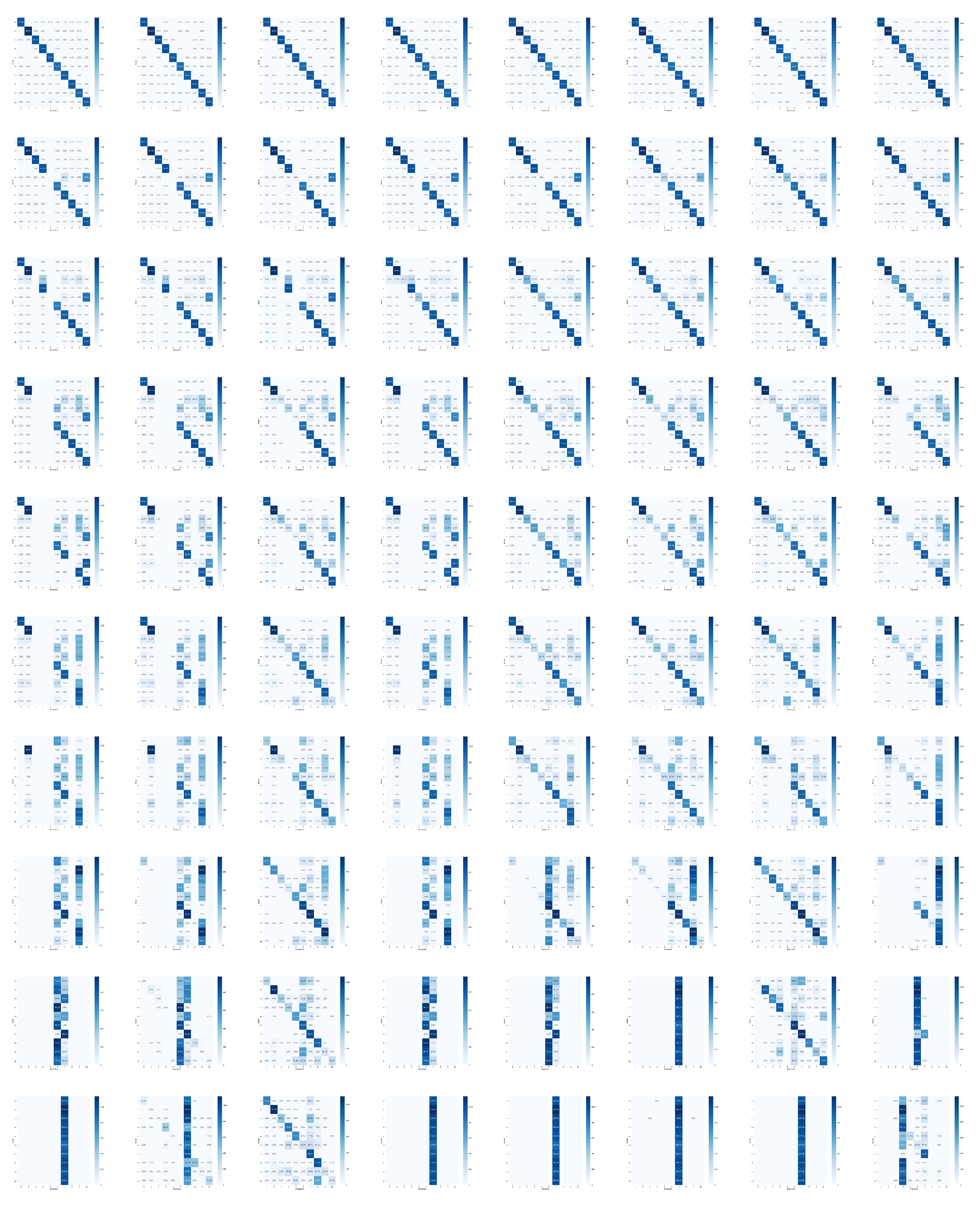
Performance.Table 1 reports the test errors (in %) with their standard errors of the eight methods in 10 training conditions over two heavy-tailed scenarios: labels with under-represented and over-represented minorities. In the balanced scenario, the proposed regularity-based method doesn’t show clear advantages over existing methods, but still manages to perform the classification tasks without major deficits. In both the “rare minority��? and “highly imbalanced��? scenarios, regularity-based methods performs the best in all groups, suggesting that the proposed method successfully constrained the model to allocate learning resources to the “special cases��? which are rare and out of normal range, while the BN and WN fail to learn it completely (ref. confusion matrices in the
Appendix B.2). We observe that, In certain cases, like n = 0, 8 and 9 (“balanced��? or “dominant oligarchy��?), some of the baselines are doing better than RN. However, that is expected because those are the three cases in the ten scenarios that the dataset is more “regular��? (or homogenous in regularity), and the benefit from normalizing against the regularity is expected to be minimal. For instance, in the “dominant oligarchy��? scenario, LN performs the best, dwarfing all other normalization methods, likely due to its invariance to data rescaling but not to recentering. However, as in the case of
, LN + RN performs considerably well, with performance within error bounds to that of LN, beating other normalization methods by over 30%. On the other hand, if we look at the test accuracy results in the other seven scenarios, especially in the highly imbalanced scenarios (RN variants over BN/WN/baseline for around 20%), they should provide promises in the proposed approach ability to learn from the extreme regularities.
We observe that LN also manages to capture the features of rare classes reasonably well in other imbalanced scenarios, comparing to BN, WN and baseline. The hybrid methods RLN and LN + RN both display excellent performance in imbalanced scenarios, suggesting that combining regularity-based normalization with other methods is advantageous, as their imposed priors are in different dimensions and subspaces. This also brings up an interesting concept in applied statistics, the “no free lunch��? theorem. LN, BN, WN and the proposed regularity-based normalizations are all developed under different inductive bias that the researchers impose, which should yield different performance in different scenarios. In our case, the assumption that we make, when proposing the regularity-based approach, is that in real life, the distribution of the encounter of the data samples are not necessarily i.i.d, or uniformly distributed, but instead follows irregularities unknown to the learner. The data distribution can be imbalanced in certain learning episodes, and the reward feedback can be sparse and irregular. This inductive bias motivates the development of this regularity-based method.
The results presented here mainly deal with the short term domain to demonstrate how regularity can significantly speed up the training. The long term behaviors tend to converge to a balanced scenario since the regularities of the features and activations will become higher (not rare anymore), with the normalization factors converging to a constant in a relative sense across the neurons. As a side note, despite the significant margin of the empirical advantages, we observe that regularity-based approach offers a larger standard deviation in the performance than the baselines. We suspect the following reason: the short-term imbalanceness should cause the normalization factors to be considerably distinct across runs and batches, with the rare signals amplified and common signals tuned down; thus, we expect that the predictions to be more extreme (the wrong more wrong, the right more right), i.e., a more stochastic performance by individual, but a better performance by average. We observe this effect to be smaller in the long term (when the normalization factors converge to a constant relatively across neurons). Future further analysis might help us fully understand these behaviors in different time scales (e.g., the converging performance over 100 epochs).
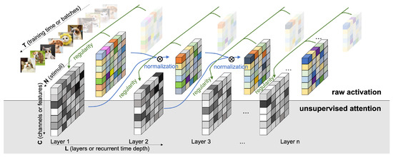
Probing the network with the unsupervised attention mechanism.
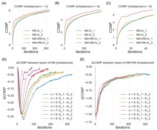
Figure 6A–C demonstrate three steoretypical COMP curves in the three imbalanced scenarios. In all three cases, the later (or higher) layer of the feedforward neural net adopts a higher model complexity. The additional regularity normalization seems to drive the later layer to accommodate for the additional model complexities due to the imbalanced nature of the dataset, and at the same time, constraining the low-level representations (earlier layer) to have a smaller description length in the implicit space. This behaviors matches our hypothesis how this type of regularity-based normalization can extract more relevant information in the earlier layers as inputs to the later ones, such that later layers can accommodate a higher complexity for subsequent tasks.
Figure 6D,E compare the effect of imbalanceness on the COMP difference of the two layers in the neural nets with or without RN. We observe that when the imbalanceness is higher (i.e.,
n is smaller), the neural net tends to maintains a significant complexity difference for more iterations before converging to a similar levels of model complexities between layers. On the other hand, the regularity normalization constrains the imbalanceness effect with a more consistent level of complexity difference, suggesting a possible link of this stable complexity difference with a robust performance in the imbalanced scenarios.
7.2. The Classic Control Problem in OpenAI Gym with Deep Q Networks (DQN)
We further evaluate the proposed approach in the reinforcement learning problem, where the rewards can be sparse. For simplicity, we consider the classical deep Q network (DQN) [
32] and test it in the OpenAI Gym’s LunarLander and CarPole environments [
33] (see
Appendix C.1 for the neural network setting and game setting). We evaluate five agents (DQN, +LN, +RN, +RLN, +RN+LN) by the final scores in 2000 episodes across 50 runs.
Performance. As in
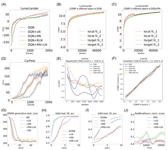
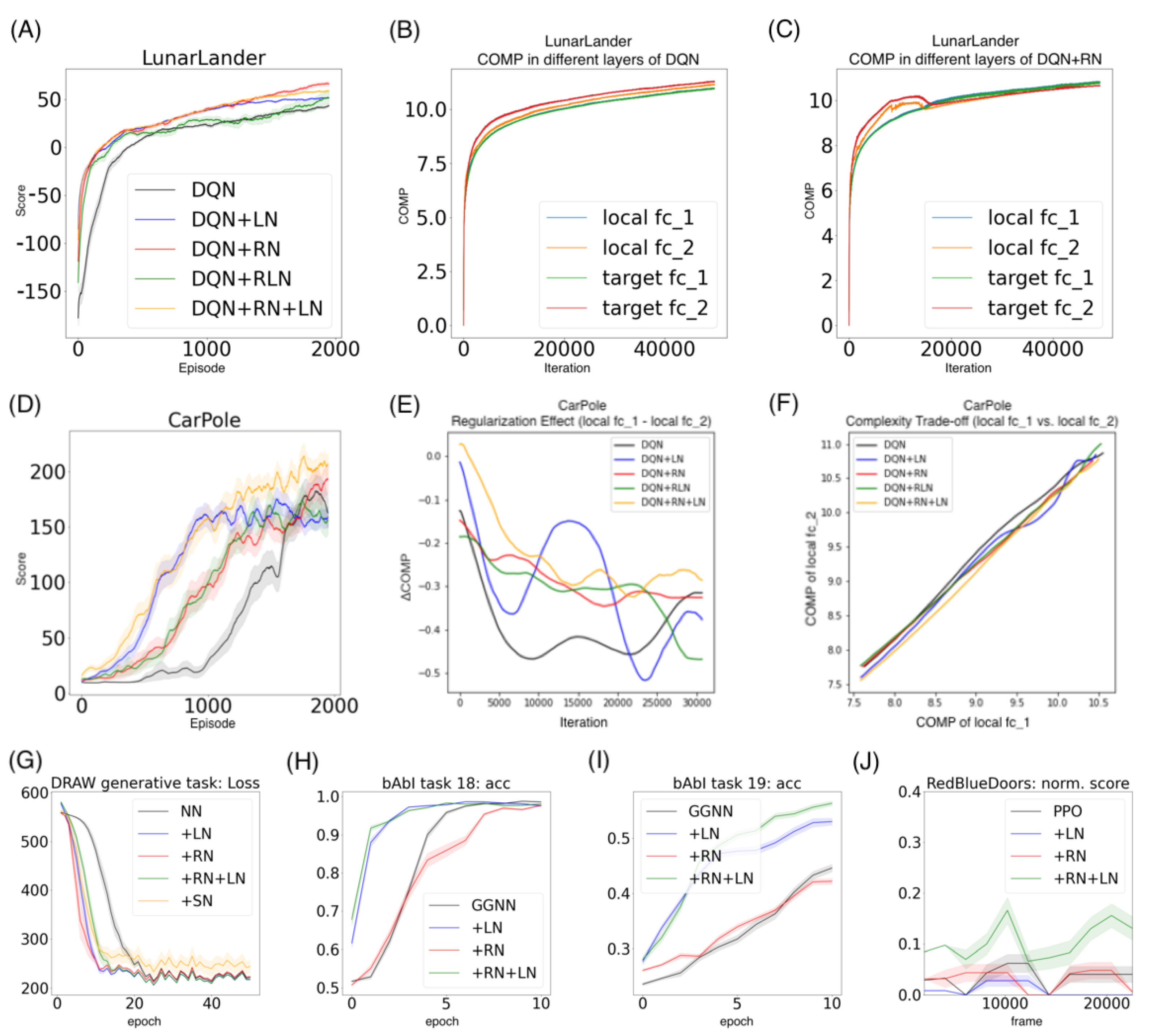
Figure 7A, in the LunarLander environment, DQN + RN (66.27 ± 2.45) performs the best among all five agents, followed by DQN + RN + LN (58.90 ± 1.10) and DQN+RLN (51.50 ± 6.58). All three proposed agents beat DQN (43.44 ± 1.33) and DQN-LN (51.49 ± 0.57) by a large marginal. The learning curve also suggests that taking regularity into account speed up the learning and helped the agents to converge much faster than the baseline. Similarly in the CarPole environment, DQN + RN + LN (206.99 ± 10.04) performs the best among all five agents, followed by DQN + RN (193.12 ± 14.05), beating DQN (162.77 ± 13.78) and DQN + LN (159.08 ± 8.40) by a large marginal (
Figure 7D). These numerical results suggests the proposed method has the potential to benefit the neural network training in reinforcement learning setting. On the other hand, certain aspects of these behaviors are worth further exploring. For example, the proposed methods with highest final scores do not converge as fast as DQN + LN, suggesting that regularity normalization resembles adaptive learning rates which gradually tune down the learning as scenario converges to stationarity.
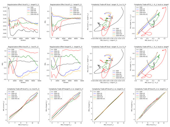
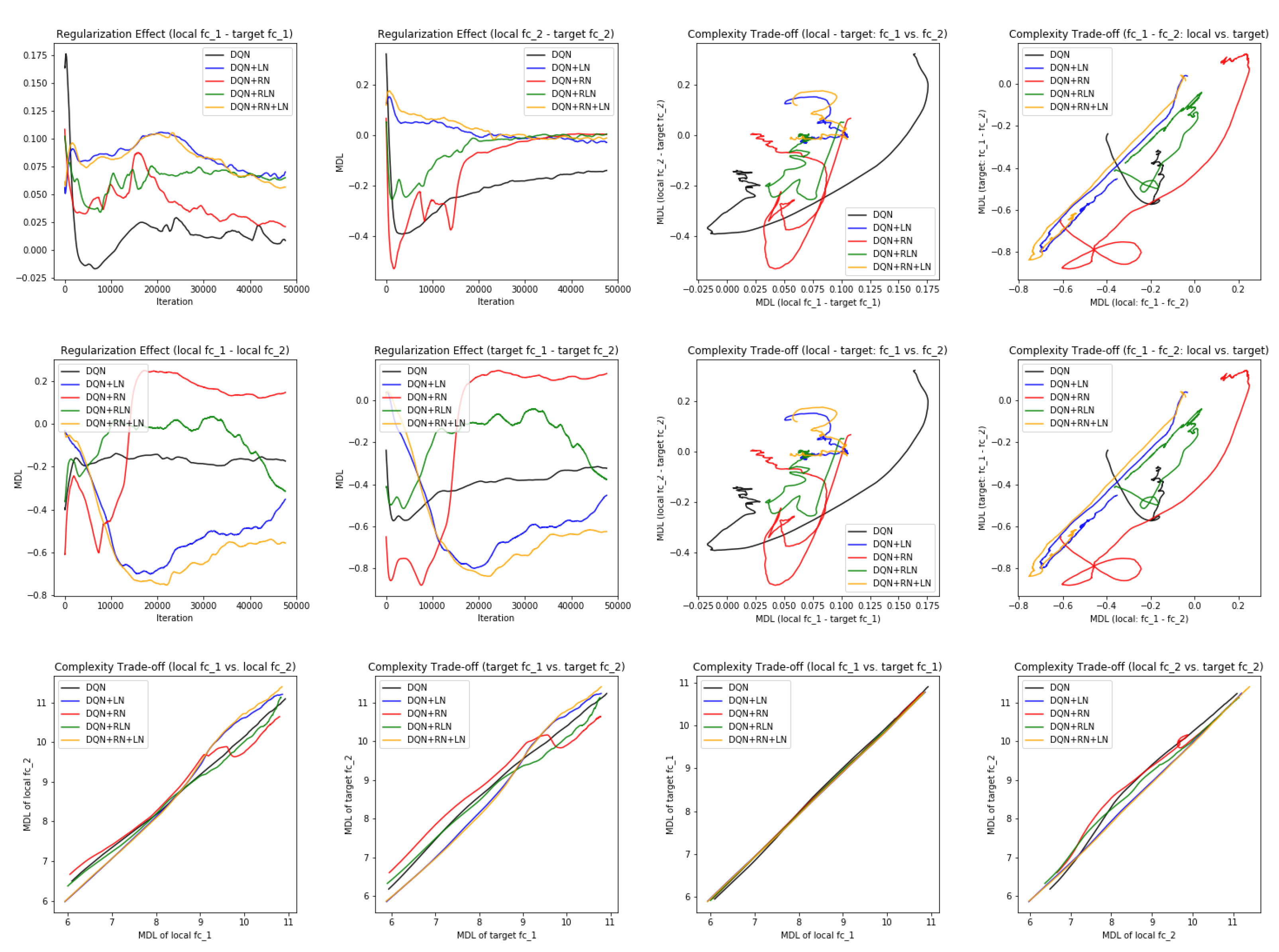
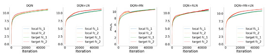
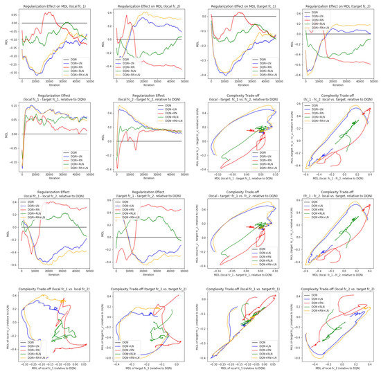
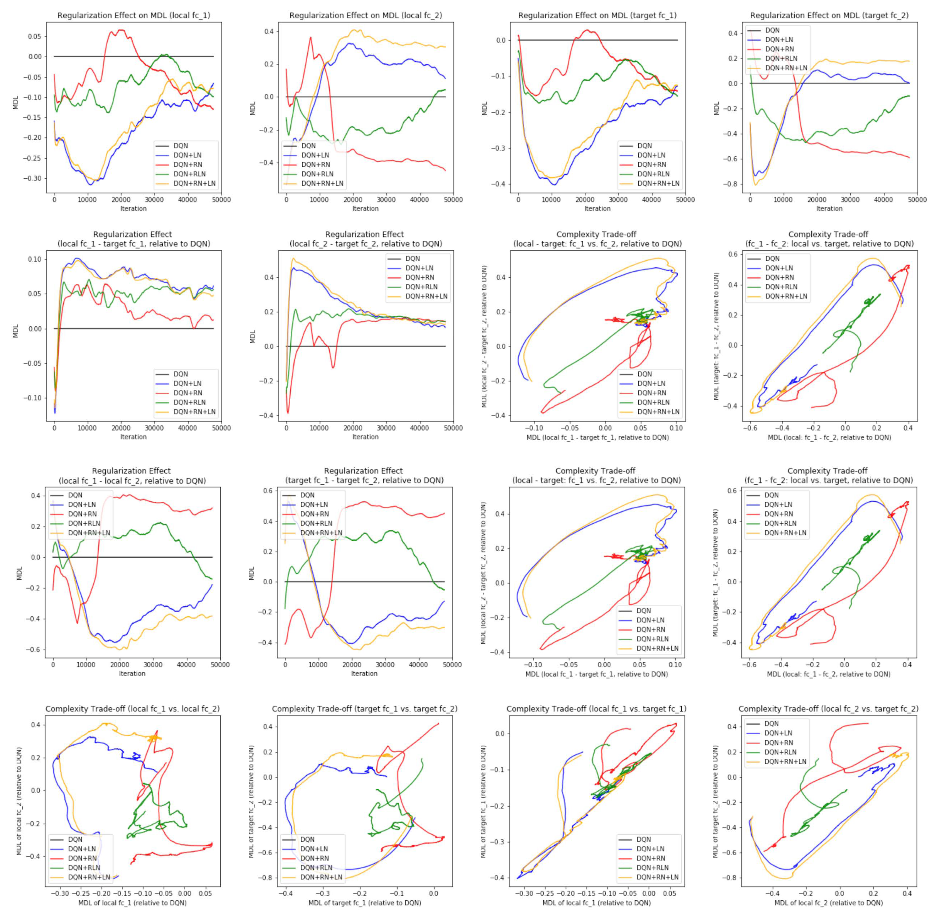
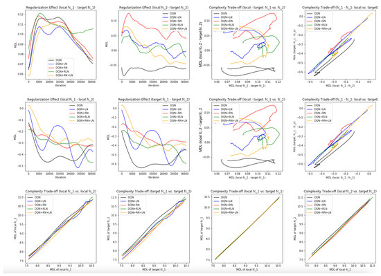
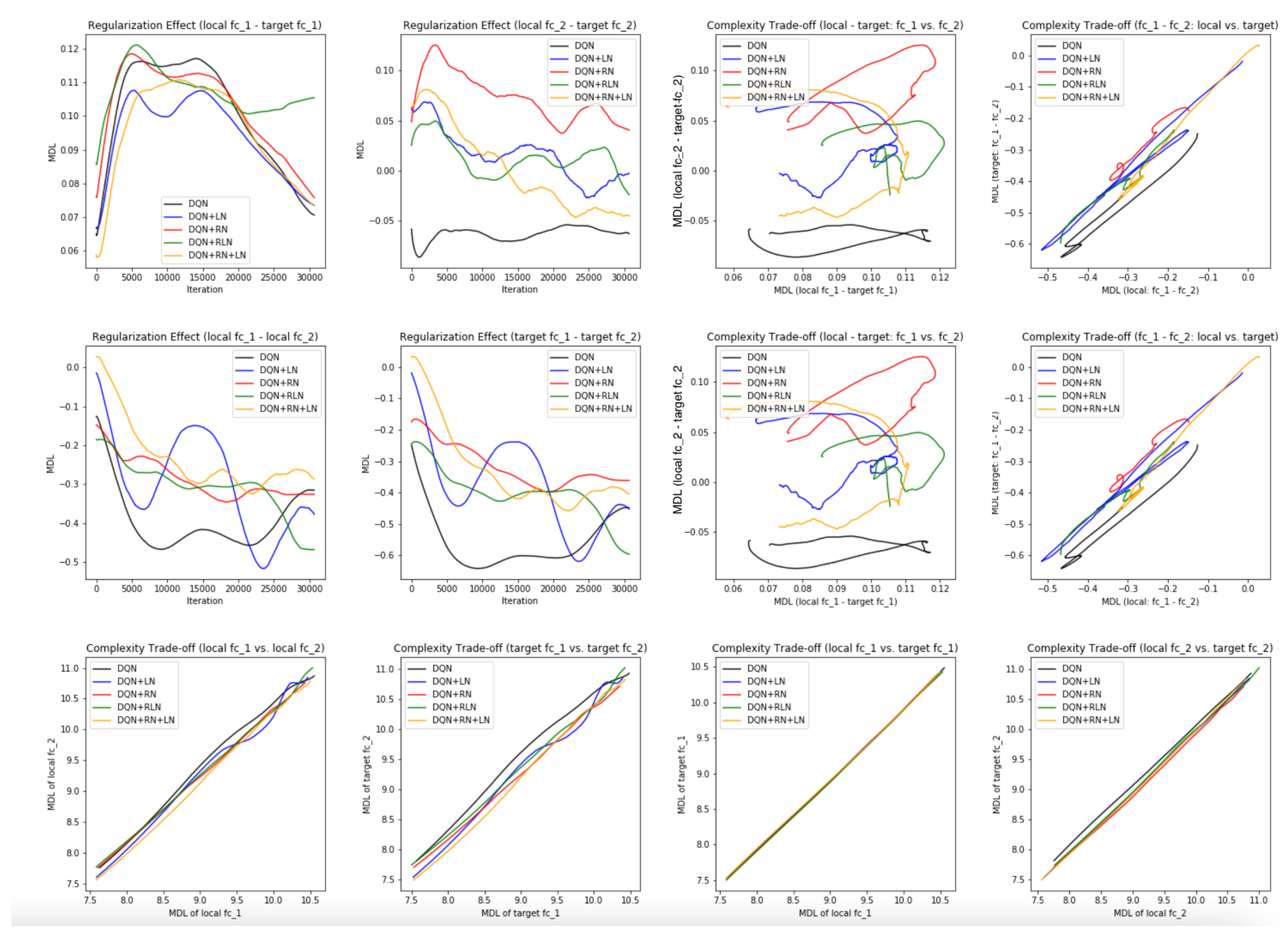
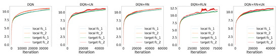
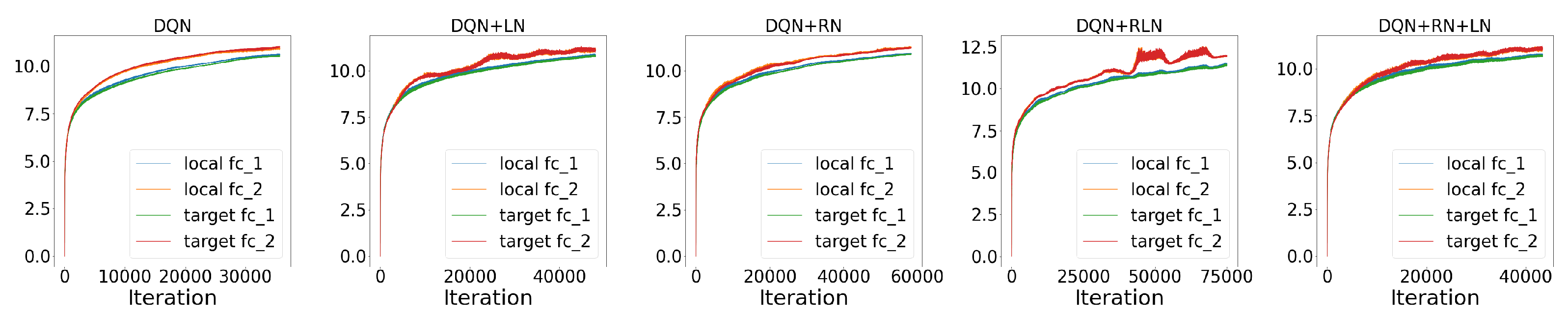
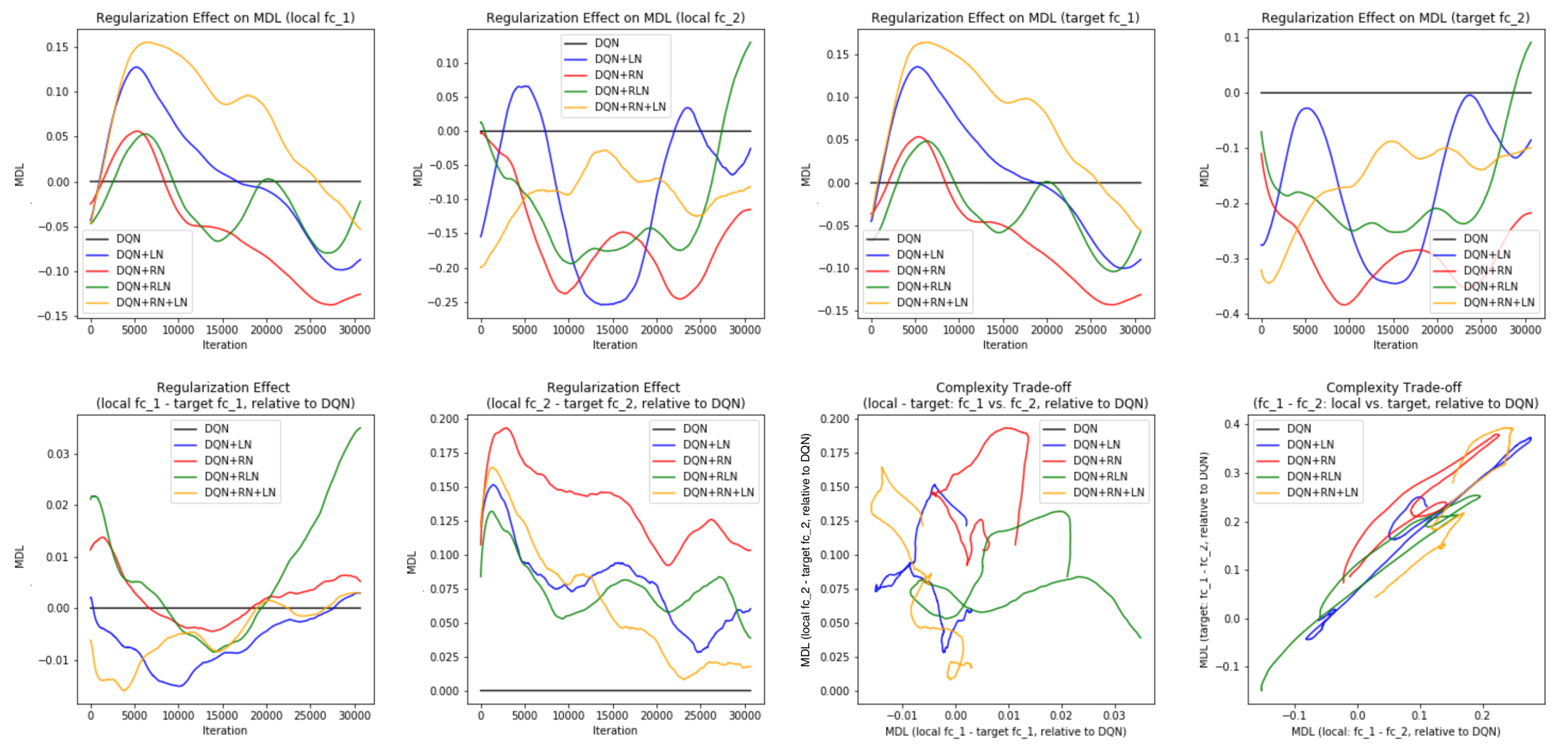
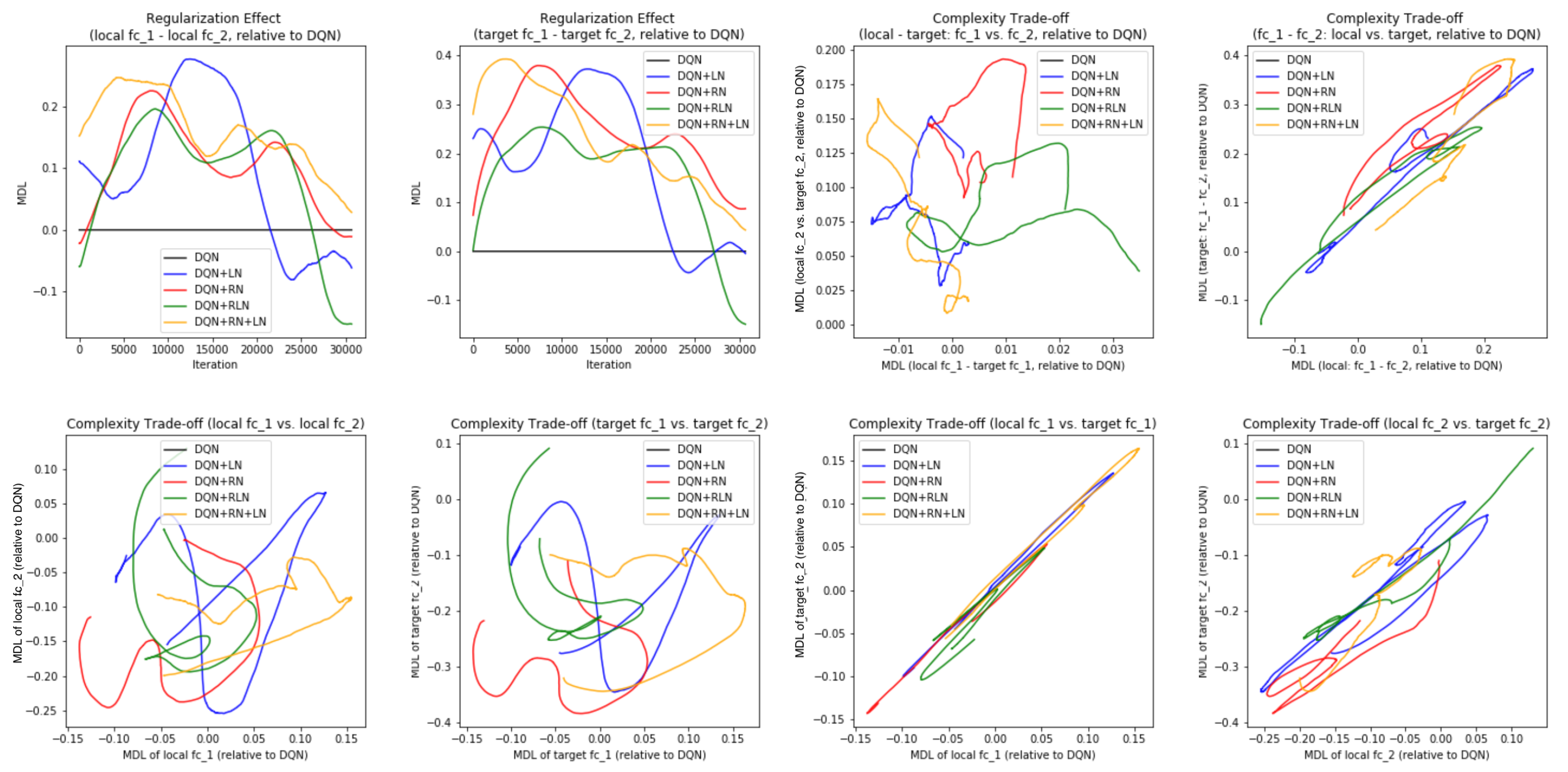
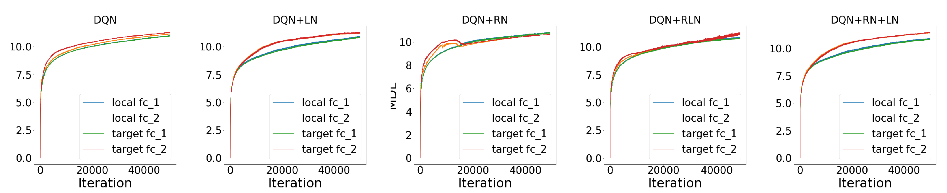
Probing the network with the unsupervised attention mechanism. As shown in
Figure 7B,C, the DQN has a similar COMP change during the learning process to the ones in the computer vision task. We observe that the COMP curves are more separable when regularity normalization is installed. This suggests that the additional regularity normalization constrains the earlier (or lower) layers to have a lower complexity in the implicit space and saving more complexities into higher layer. The DQN without regularity normalization, on the other hand, has a more similar layer 1 and 2. We also observe that the model complexities COMP of the target networks seems to be more diverged in DQN comparing with DQN+RN, suggesting the regularity normalization as a advantageous regularization for the convergence of the local to the target networks.
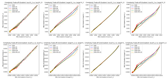
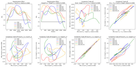
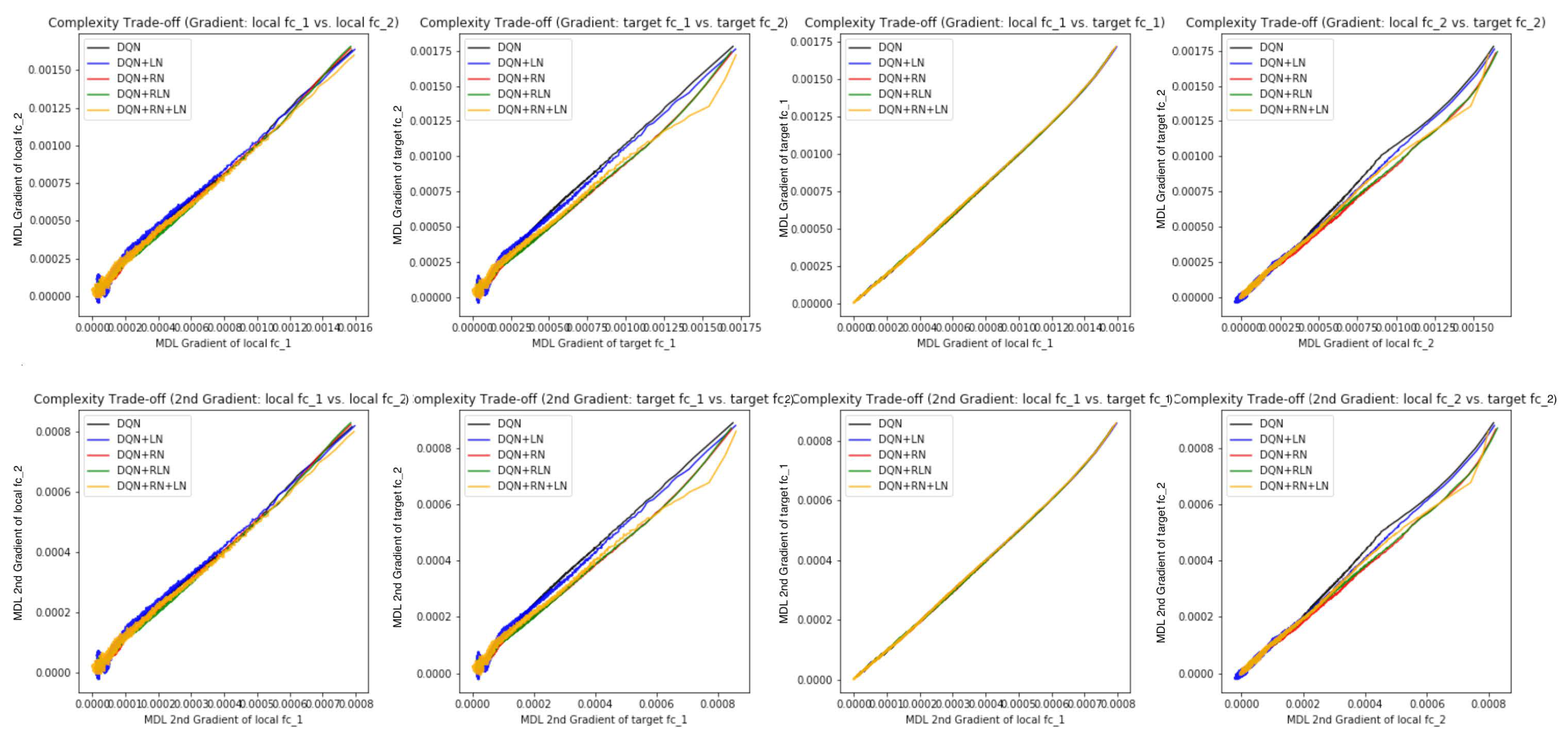
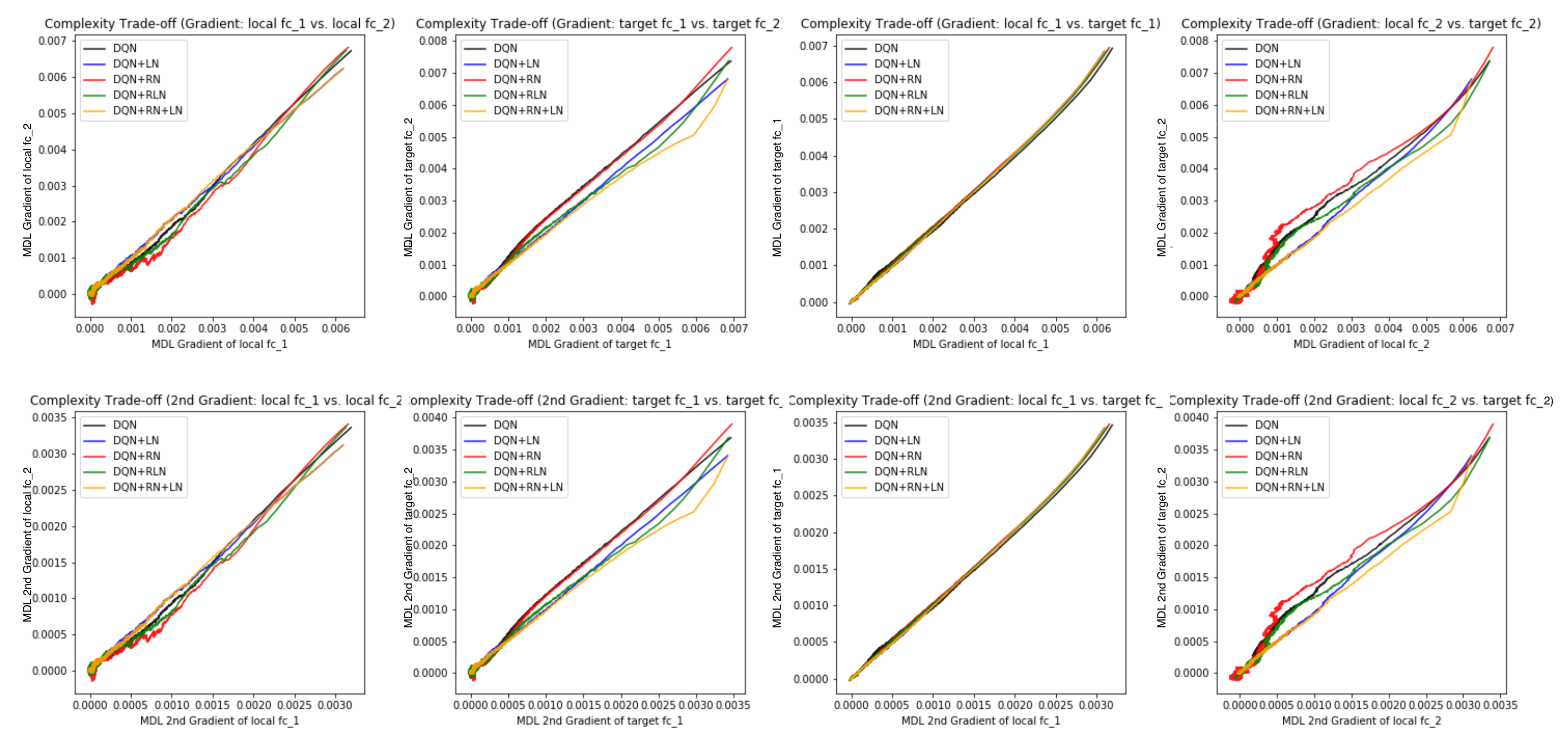
Figure 7E,F offer some intuition why this is the case: the DQN+RN (red curve) seems to maintain the most stable complexity difference between layers, which stabilizes the learning and provides a empirically advantages trade-off among the expressiveness of layers given a task (see
Appendix C.3 for a complete spectrum of this analysis).


