2241 Features of the stress field at the surface of a flush shrink-fit shaft R J H Paynter1∗ , D A Hills1 , and J R Barber2 1 Department of Engineering Science, University of Oxford, Oxford, UK 2 Department of Mechanical Engineering, University of Michigan, Ann Arbor, Michigan, USA The manuscript was received on 20 October 2008 and was accepted after revision for publication on 6 April 2009. DOI: 10.1243/09544062JMES1403 Abstract: The state of stress induced by a shrink-fitted circular shaft in an elastically similar half-space, positioned so that the end of the shaft is flush with the remainder of the free surface, is studied. At deep interior points the classical plane strain (Lamé) solution obtains, and the transition to the free surface state is found. It is found that a residual interfacial axial shear develops and the coefficient of friction needed to ensure adhesion along the interface is found. The effect of slip when a lower coefficient of friction is present is also found as a solution to an integral equation. Keywords: shrink fit, end-effects, Lamé solution 1 INTRODUCTION The shrink fit remains a standard, reliable way of fastening substantial wheels and other fittings onto shafts, and is frequently used. The usual way of deciding the degree of interference required is to use the plane Lamé ‘thick cylinder’ calculation, found in many undergraduate textbooks (see for example, reference [1]), and which explicitly gives the connection between the amount of interference and the contact pressure produced. An estimate of the minimum coefficient of friction at the interface is also needed in order to permit the driving torque, which may be transmitted to be estimated. Because the Lamé solution is strictly two-dimensional in nature it can only be used, accurately, under conditions of transverse plane strain (i.e. well away from any free surface) and the question of how end effects might lead to a modification of the interface pressure, and hence introduce the possibility of slip and attendant fretting, arises. 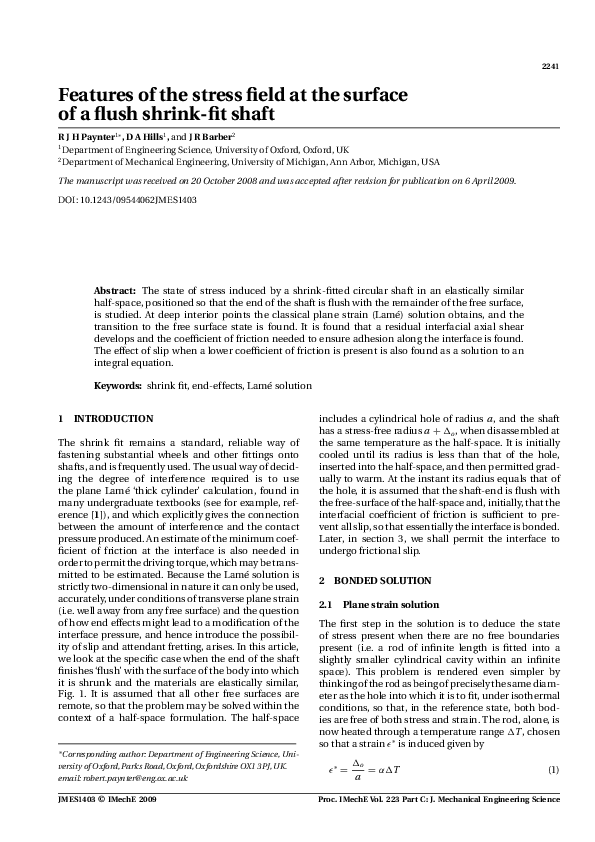In this article, we look at the specific case when the end of the shaft finishes ‘flush’ with the surface of the body into which it is shrunk and the materials are elastically similar, Fig. 1. It is assumed that all other free surfaces are remote, so that the problem may be solved within the context of a half-space formulation. The half-space ∗ Corresponding includes a cylindrical hole of radius a, and the shaft has a stress-free radius a + o , when disassembled at the same temperature as the half-space. It is initially cooled until its radius is less than that of the hole, inserted into the half-space, and then permitted gradually to warm. At the instant its radius equals that of the hole, it is assumed that the shaft-end is flush with the free-surface of the half-space and, initially, that the interfacial coefficient of friction is sufficient to prevent all slip, so that essentially the interface is bonded. Later, in section 3, we shall permit the interface to undergo frictional slip. 2 BONDED SOLUTION 2.1 Plane strain solution The first step in the solution is to deduce the state of stress present when there are no free boundaries present (i.e. a rod of infinite length is fitted into a slightly smaller cylindrical cavity within an infinite space). This problem is rendered even simpler by thinking of the rod as being of precisely the same diameter as the hole into which it is to fit, under isothermal conditions, so that, in the reference state, both bodies are free of both stress and strain. The rod, alone, is now heated through a temperature range T , chosen so that a strain ǫ ∗ is induced given by author: Department of Engineering Science, Uni- versity of Oxford, Parks Road, Oxford, Oxfordshire OX1 3PJ, UK. email: robert.paynter@eng.ox.ac.uk JMES1403 © IMechE 2009 ǫ∗ = o = αT a (1) Proc. IMechE Vol. 223 Part C: J. Mechanical Engineering Science 2242 R J H Paynter, D A Hills, and J R Barber surface of the shaft, urs (a), is given by 1 urs = ǫθs θ = [−p1 (1 − ν) + νp2 ] + ǫ ∗ a E (5) and the unknown axial pressure is found from the plane strain condition, i.e. s 0 = ǫzz = Fig. 1 Geometry plug of radius a, in a half-space z > 0 where α is the coefficient of thermal expansion and this generates a state of stress within the assembly. As there are no gradients in the z direction, a state of plane strain exists, and hence ǫzz = 0 in both bodies. Exterior to the rod, the state of stress, from Lamé’s solution, is given by 2 σrr σθ θ a =− =− 2, p1 p1 r ra (2) where p1 is the interfacial contact pressure between the rod and the cavity wall, and it will be noted that, even under plane strain, because the material is under pure shear, σzz = 0. The radial displacement at the bore, urh (a), is given by p1 (1 + ν) urh = ǫθhθ = a E (3) where ν is the Poisson’s ratio and E is the Young’s modulus. Turning to the shaft, we know that, because of the pressure associated with contact with the bore, p1 , this suffers a constant state of stress everywhere, given by σrr σθ θ = = −1 p1 p1 (4) Suppose that it is also subject to a constant axial pressure, σzzs = −p2 , so that the radial displacement of the 1 [−p2 + 2νp1 ] + ǫ ∗ E (6) while continuity in the radial direction requires that urs (a) = urh (a) (i.e. equations (3) and (5)) mean that 2p1 = p2 = −σzz = Eǫ ∗ 1−ν (7) and thus ⎧ 1 ⎪ ⎪ ⎨− 2 σrr (1 − ν) = 2 ⎪ Eǫ ∗ ⎪ ⎩− a 2r 2 ra (8) r>a We will use σo = Eǫ ∗ /(1 − ν), the axial stress, as a reference value in subsequent normalization. 2.2 Disc of pressure Now introduce a free surface, along the plane z = 0. There are no shear tractions anywhere along this plane, and the direct traction already vanishes when r > a. It therefore remains only to cancel the disc of constant pressure, p2 , present on r  a. This stress field has been found by first finding the Papkovich–Neuber potential function for an axial traction with uniform distribution on an internal circular disc in a full-space, as presented by Paynter et al. [2]. This solution was then transformed, by means of a method developed by Aderogba [3], to a halfspace problem with the disc of pressure set at the surface; the resulting formulae are presented in reference [4] in terms of Lipschitz–Hankel integrals which may, in turn, be given in terms of complete elliptic integrals. The two stress components relevant to this investigation are ⎡ σrr (a, r, z) z ⎢ [2ar(2 − k 2 )(3 − 2ν) − k 2 r 2 (3 + 2ν) + a 2 k 2 (1 − 2ν)]K(k 2 ) = −⎣ √ p2 4π akr 5/2 z {k 2 r − 2a(3 − 2ν)(r 2 + z 2 ) − 2a 3 (3 − 2ν) − a 2 r(k 2 − 12 + 8ν)}E(k 2 ) √ 2 a(a − 2ar + r 2 + z 2 ) ⎧ ⎤ 1 + 2ν ⎪ ⎪ r < a⎥ ⎨ 2 2 kz[r (1 + 2ν) + a (1 − 2ν)] r − a 2 ⎥
(h, k 2 ) + + √ ⎦ 5/2 ⎪ a 2 (1 − 2ν) r +a 4πr a ⎪ ⎩− r > a 2r 2  2 2 σrz (a, r, z) z (k − 2) 2 2 =− E(k ) − K(k ) p2 2πr (a + r)2 + z 2 (k 2 − 1) + 2πr 3/2 k Proc. IMechE Vol. 223 Part C: J. Mechanical Engineering Science (9) (10) JMES1403 © IMechE 2009 Features of the stress field at the surface of a flush shrink-fit shaft Fig. 2 Contours of stress fields, adhered case: (a) radial stress and (b) shear stress where k=  h= 4ar (r + a)2 4ar , (r + a)2 + z 2 k′ = 1 − k2 (11) and K (·), E(·), and (·) are, respectively, the complete elliptic integrals of the first, second, and third kinds [5]. It may be noted that the term including (h, k 2 ) is discontinuous across r = a, but this discontinuity is removed by the final term in the expression for σrr . 2.3 Overall solution The overall solution for the fully adhered plug is thus the sum of the effect expansion (equation (8)), minus the corrective term for pressure at the free surface (equations (9) and (10)). The contour plots in Fig. 2 show the overall radial and shear stress fields. In this and all other example evaluations a Poisson’s ratio of 0.3 has been used. The state of stress is smooth and continuous everywhere, except where the interface meets the surface where an interesting feature arises. There is a discontinuity in the radial stress given by  σrr (1 − ν)  Eǫ ∗  z=0 = ⎧ ⎪ ⎨ν The shear stress σrz on the surface r = a tends to a non-zero limit as z → 0, though the complementary shear stress σzr is of course zero at this point since the surface z = 0 is traction-free. In fact the stress field, though everywhere bounded, has an unbounded derivative at (a, 0) and the values of the stress components obtained at that point depend on the inclination of the line along which it is approached (see Barber [6], section 11.1). Note that these discontinuities arise only strictly at the point (a, 0) and at all other points the stress is continuous. The radial stress is plotted as a function of radius in Fig. 3 at the surface (z = 0), under plane strain conditions (z = ∞) and for a selection of depths (z/a = 1/20, 1/4, 1). Note that the radial stress at the surface on the shaft end is tensile for positive values of Poisson’s ratio (see equation (12)). Although the stress gradients are severe at the surface, at depths of greater than two diameters the stresses tend to their plane strain values. r<a 2 ⎪ ⎩− a (1 − ν) r > a r2 (12) The magnitude of the discontinuity is equal to the axial stress in the shaft at infinite depth. JMES1403 © IMechE 2009 2243 Fig. 3 Radial stress versus radial position. At the surface (z = 0), plane strain (z = ∞), and at example depths: z/a = a/20, a/4, 1 Proc. IMechE Vol. 223 Part C: J. Mechanical Engineering Science 2244 R J H Paynter, D A Hills, and J R Barber For analysis of the shaft or plug we are most interested in the stress arising along the interface (r = a), which is given by  σrr (1 − ν)  Eǫ ∗  r=a  2 z [4a (1 − 2ν) + z 2 (3 − 2ν)]K(k 2 ) √ 2a 2 π 4a 2 + z 2  1 (13) −[2a 2 (5 − 4ν) + z 2 (3 − 2ν)]E(k 2 ) + ν − 2  σrz (1 − ν)  1 [z 2 K(k 2 ) = √  ∗ 2 + z2 Eǫ aπ 4a r=a = − (2a 2 + z 2 )E(k 2 )] (14) The values at the surface found by approaching along this line are given by these formulae and then take the limit z → 0, which gives  σrr (1 − ν)  1 =ν−  ∗ Eǫ 2 r=a,z=0  1 σrz (1 − ν)  = Eǫ ∗ r=a,z=0 π (15) (16) which, for the radial stress, is the average of the values either side of the discontinuity (equation (12)). This represents the complete solution to the problem, providing only that the coefficient of friction f is sufficient to maintain conditions of stick throughout the interface, in other words, that the traction ratio |σrz |/(−σrr ) does not exceed f anywhere along the interface. This ratio and the individual traction components are presented in Fig. 4 as a function of depth along the interface. It may be seen that the most critical point is just below the surface, where, for ν = 0.3, the maximum lies at z/a = 0.0227, and the ratio equals −1.616 whereas, at the surface, it is −1.592. Of course, for practical values of friction coefficient the interface would slip. Fig. 4 3 FRICTIONAL SLIP When the coefficient of friction is insufficient to maintain complete adhesion, a region of slip will develop, whose extent we wish to find. In order to do this we will deploy an array of glide dislocations along the slipping interface, to restore the Coulomb condition. A prerequisite is a knowledge of the state of stress within a half-space because of a dislocation loop, of radius a, having a Burgers vector in the z direction, of magnitude bz , and positioned at (a, d). The path cut must lie along the line of slip (i.e. lie along the cylindrical surface r = a, 0  z  d) and a solution to this problem has recently been found [4]. We therefore know the functions z Gri (ζ , z), defined by σri (z) = z Gri (ζ , z)bz (ζ ), i = r, z (17) and hence can write down the following two integral equations describing the tractions along the interface as ∞ 0 (18) σrr (z) = σrr (z) + z Grr (ζ , z)Bz (ζ )dz 0 σrz (z) = σrz0 (z) + ∞ z Grz (ζ , z)Bz (ζ )dz (19) 0 where σrj0 is the fully stuck (or bilateral) solution given above and Bz (·) represents the dislocation density, (= dbz /dz). If the slip region penetrates to a depth c, and the coefficient of interfacial friction is f , along the interface we know that 0zc σrz (z) = −f σrr (z), (20) and hence we arrive at the following singular integral equation, in terms of the dislocation density σrz0 (z) −f σrr0 (z) = c 0 [z Grz (ζ , z) − f z Grr (ζ , z)]Bz (ζ )dz (21) A ‘bounded both ends’ solution is required for the dislocation density, and this provides the additional side Stresses at the interface radius (r = a) versus depth z/a. Adhered solution: (a) pressure and shear and (b) traction ratio |σrz |/(−σrr ) Proc. IMechE Vol. 223 Part C: J. Mechanical Engineering Science JMES1403 © IMechE 2009 Features of the stress field at the surface of a flush shrink-fit shaft Fig. 5 Friction coefficient for a given slip length condition needed to establish consistent values of the friction coefficient for a given extent of slip, c/a. The integral equation is treated using a Gauss–Chebyshev numerical quadrature appropriate to this type of kernel, a detailed description of which may be found in reference [7]. This quadrature gives greatest detail to the ends of the integration interval, as required in our problem that exhibits high gradients of stress at the surface and at the point of stick-slip transition. 3.1 Results with slip The main result is the relationship between depth to which slip penetrates and the coefficient of friction. This is shown in Fig. 5, with each point representing a solution of the integral equation (equation (21)). As Fig. 6 Fig. 7 2245 would be expected the length of the slip zone increases with reducing friction coefficient. Specific examples are given to show the tractions along the interface. In Fig. 6, with a friction coefficient of 1.0, the slip extends to 0.674a. There is little effect on the overall radial stress distribution, with only a small reduction in the magnitude. The shear in the slip zone is affected substantially in the slipping region as it is constrained to follow the form of the radial stress (equation (20)) to the point of transition to stick. The peak shear traction now occurs here instead of at the surface. With a friction coefficient of 0.3 (Fig. 7) the slip extends to 3.31a. There is a significant reduction in the radial stress well within the half-space, but near the surface there is an increase in radial pressure. The plots in Fig. 8 show the radial and shear stress fields in this case; the shift of the concentration of shear stress is clear and the magnitude has decreased (note the contour labels). The magnitude of the radial stress anomaly at the surface has decreased, such that the surface is now in compression. At very low coefficients of friction the modification of the radial pressure by slip is marked. It is easy to find the limiting relationship for a vanishingly small coefficient of friction analytically, by setting the axial stress p2 in equation (5) to zero, whereupon the relationship between the interfacial contact pressure and dimensionless interference is seen to be given by σrr /σo = −(1 − ν)/2, and, of course, this solution is exact at all Friction coefficient = 1.0 and slip length = 0.674 (dashed lines show bilateral adhered solution). (a) Radial pressure and (b) shear traction Friction coefficient = 0.3 and slip length = 3.31a. (a) Radial pressure, (b) shear traction JMES1403 © IMechE 2009 Proc. IMechE Vol. 223 Part C: J. Mechanical Engineering Science 2246 R J H Paynter, D A Hills, and J R Barber Fig. 8 Fig. 9 Contours of stress fields: friction coefficient = 0.3 and slip length = 3.31a. (a) Radial stress and (b) shear stress Friction coefficient = 0.0233 and slip length = 50a (dashed lines show bilateral adhered solution). Radial pressure depths within the half-space. In Fig. 9, the slip zone was set to 50a and the corresponding friction coefficient found to be 0.0233. The radial pressure tends to the limiting value of the frictionless case at the surface, namely 0.35σo for ν = 0.3. A small, finite coefficient of friction fixes the depth at which the axial displacements of the shaft and pocket are fixed, and hence the projection of the shaft when the strain is relaxed may be found. For mild steel (E = 210 GPa, ν = 0.3, and σY = 300 MPa), which remains elastic ǫ ∗ cannot exceed about 10−3 so that the plug would protrude by about a/20, and the ‘flush surface’ idealization is justified. the radial stress is not uniquely defined, but depends on the direction of approach. Immediately external to the shaft the radial stress is given by σrr /σo = −(1 − ν), and immediately inside it is given by σrr /σo = ν (i.e. it is in tension). The practical implication of this result is that the contact pressure will fall off towards the free end, by an amount dependent on the coefficient of friction, and with a lower bound given by the second of the equations just quoted (i.e. for a material having a Poisson’s ratio of 0.3, to 40 per cent of the plane strain value). This contrasts with the value implied by a naive assumption of plane stress which incorrectly implies an increase in local contact pressure to 142 per cent of the plane strain value. In absence of external loading the coefficient of friction would have to exceed about 1.6 to eliminate completely all axial slip. In most practical cases slip will most certainly ensue and depth of penetration of slip is quite marked. For example if the coefficient of friction is only 0.3 axial slip will penetrate to as far as just over three times the plug radius. Even the coefficient of friction is as high as one the slip extends to about 0.67 of the plug radius. The presence of external load can be expected to extend slip further but this cannot easily be quantified within this formulation. REFERENCES 4 CONCLUSIONS The variation of radial contact stress arising between an elastic cylindrical shaft and a slightly undersized hole in an elastically similar half-space has been found. The stress field is unusual insofar as at the point where the interface comes to the free surface 1 Zhang, L. Solid mechanics for engineers, 2001 (Palgrave, Basingstoke, UK). 2 Paynter, R. J. H., Hills, D. A., and Korsunsky, A. M. The effect of path cut on Somigliana ring dislocation elastic fields. Int. J. Solids Struct., 2007, 44, 6653–6677. 3 Aderogba, K. Eigenstresses in a semi-infinite solid. Math. Proc. Camb. Philos. Soc., 1976, 80, 555–562. Proc. IMechE Vol. 223 Part C: J. Mechanical Engineering Science JMES1403 © IMechE 2009 Features of the stress field at the surface of a flush shrink-fit shaft 4 Paynter, R. J. H. and Hills, D. A. The effect of path cut on Somigliana ring dislocation elastic fields in a half-space. Int. J. Solids Struct., 2009, 46, 412–432. 5 Abramowitz, M. and Stegun, I. A. Handbook of mathematical functions, 1964 (Dover Publications Inc., New York, USA). 6 Barber, J. R. Elasticity, 2002 (Kluwer Academic Publishers, Dordrecht, The Netherlands). 7 Hills D. A., Kelly, P. A., Dai, D. N., and Korsunsky, A. M. Solution of crack problems; the distributed dislocation technique, 1996 (Kluwer Academic Publishers, Dordrecht, The Netherlands). Notation E f h, k Jμ,ν;λ K(k 2 ), E(k 2 ),
(h, k 2 ) p1 , p2 r, z ur α o APPENDIX a Bz Gri radius of shaft axial ring dislocation density Young’s modulus coefficient of friction JMES1403 © IMechE 2009 ǫ∗ ǫzz , ǫθθ ν σrr , σzz , σθθ , σrz 2247 stress influence functions of ring dislocations arguments of elliptic integrals Lipschitz–Hankel function complete elliptic integrals of the first, second, and third kind radial and axial pressure in the shaft of the plane strain solution radial and axial axisymmetric cylindrical coordinates radial displacement coefficient of thermal expansion interference of shaft and hole at equal temperature thermal or misfit strain axial and tangential strain Poisson’s ratio for the elastic material (=0.3 in example calculations) radial, axial, tangential, and shear stress Proc. IMechE Vol. 223 Part C: J. Mechanical Engineering Science