Power Control Scheme in Very Fast Fading Wireless Communication Systems Concerning the Effect of Noise and Interference Roozbeh Mohammadian Mehrzad Biguesh Wireless Comm. Laboratory, Dept. of Electrical Engineering, Engineering School, Shiraz University, P.C. 71348-51154, Shiraz, Iran biguesh@sharif.edu A BSTRACT A very efficient approach to increase the QoS and capacity of wireless communications is to control the transmit powers. The existing power control schemes are mostly designed for power adjustment in environments that the channel is varying slowly. However, when the user channels vary very fast these methods fail to properly adjust the transmit powers. For power control in such scenarios one solution is to adjust the transmit powers in order to tune the users probability of outage instead of tuning the instantaneous SINR. This paper studies the problem of power control in very fast Rayleigh fading wireless systems concerning the effect of interference and noise. We propose to minimize the total transmit power with constraints on the users outage probabilities and transmit powers bound. Then we change this problem to a geometric program which can be handled using numerical approaches. Computer simulations show the efficiency of the proposed method. 1 I. I NTRODUCTION In mobile communication environments, because of the bandwidth resource restriction the channel is reused by several users which reduces the quality of services (QoS) in these systems. Increasing the capacity and QoS is always of important interest for vendors and researchers where power control (PC) is an intelligent and very effective tool for adjusting the transmitted powers such that the users experience a predefined QoS while at the same time the total transmit power is minimized [1]. Generally, the power control schemes are divided into distributed and centralized techniques. In distributed power control (DPC), mainly the user received SINRs are used by base stations to iteratively adjust the transmitted powers so that all users finally meet the QoS requirements [1][2][3]. In centralized power control (CPC), all information about the 1 This work was partially supported by Iran Telecommunication Research Center (ITRC). users channels are collected in a central unit which determines the proper transmit powers for each user [4][5]. Usually, centralized [4][6] and distributed [1][2] power control algorithms assume quasi-stationary fading wireless channels. Thus, they consider that the channels are static within sufficient period of time and the instantaneous signal to interference ratio (SIR), signal to interference and noise ratio (SINR), or instantaneous value of some other related parameters are used as a criterion for adjusting the transmit powers to satisfy a predefined QoS for each user in the system. However, in wireless communication systems that exhibit fast variations of the channels, these methods might not always be practical [7]. There are two common methods for power control in very fast fading channel scenarios. The first one develops an algorithm that attempts to predict the channel’s behavior based on past observations of the users’ channels and then it uses those predictions to update the transmit powers. These methods require knowledge of channel’s gain and the user’s received SINR at each time instant, also some statistical information about the communication channel is required [8]. The above necessities result in a complex system and also cause a loss in bandwidth efficiency due to channel estimation phase and the related channel estimation error. The second approach is based on the knowledge of the channel’s mean gains and does not require to be updated until the channel’s mean changes [7]. These schemes either minimize the probability of fading-induced outage or they find a power control approach which bounded the outage probabilities of the users in the system. In this paper we focus on the second methods because they are more efficient and also easy to implement. We consider the problem of minimizing the total transmit power subject to outage probability constraints and bounds on individual transmit and receive powers. In section II of this paper, we describe the system model and we give a brief review of the formulations. Section III proposes the power control problem in very fast fading wireless channels and transforms it to a geometric program (GP) problem. Geometric programming is also briefly addressed in section IV. Section V contains our computer simulations and finally we conclude in section VI. II. S YSTEM M ODEL Let us consider a CDMA cellular radio system with M cells and one active user in each cell. For simplicity we assume that the ith user is connected to the ith BTS. The channels between each user in the system and all BTS are Rayleigh fading channels. This assumption is true if neither the desired nor the interference signals have direct line-of-sight components. With such channels, the power received from transmitter j by ith receiver is given by, In a noise free scenario (or the so called interference dominant case), the above outage reduces to, Y 1 Oi = 1 − γth θik Gik Pk 1 + θii Gii Pi k6=i III. P ROPOSED POWER CONTROL PROBLEM We consider a fast fading channel and for power adjustment our goal is to minimize the total transmit power subject to outage probability constraints and bounds on transmit and receive powers. Here, we propose the following problem for power control, P = arg min P Gij Fij Pj where Fij represent the Rayleigh fading and Pj is the transmit power from the jth transmitter. Additionally, the slowly varying term Gij contains the effect of propagation gain, the log-normal fading due to shadowing, and also the antenna gain between the jth transmitter and ith receiver. We assume that the coefficients Fij s are independent random variables with exponential distribution and without loss of generality we assume that they have a unity mean. For the described system it is easy to see that the ith user received SINR is, SINRi = σ2 + θ G F P Pii ii ii i k6=i θik Gik Fik Pk (1) where, σ 2 is the power of noise, θik shows the CDMA despreading gain for the signal of the kth transmitter that is captured by the ith receiver, and X θik Gik Fik Pk k6=i shows the total interference power experienced by the ith user because of the co-channel signals transmitted to other users in the system. For very fast fading channels, one can relate the quality of service (QoS) to the distribution of the received signal SINR. As an approach, in order to ensure a satisfactory QoS, the user received SINR has to be more than a predefined threshold with some sufficiently high probability. Let us define the probability of outage as, Oi = P rob{SINRi ≤ γth } Using (1) this outage probability can be expressed as, n Oi = P rob θii Gii Fii Pi ≤ γth σ 2 + o X γth θik Gik Fik Pk s.t. M X Pi (5) i=1 Oi ≤ Oimax for i = 1, . . . , M Pimax for i = 1, . . . , M for i = 1, . . . , M Pi ≤ Gii Pi > Pth where, vector P = [P1 , . . . , PM ]T contains the desired transmit powers, Oimax is the maximum allowed outage probability for ith receiver, and Pimax is the maximum transmit power of ith transmitter due to the transmitter hardware limitations. In this problem, Gii Pi > Pth guarantees a sufficiently high received signal power (in average) for proper operation of the ith receiver (this is related to the sensitivity of the user receiver)2 . The objective function in optimization problem (5) is a linear combination of the powers Pi , while the outage probabilities Oi are nonlinear functions of transmit powers Pi . Consequently, the existing convex optimization methods can not be directly used to solve the above problem. However, (5) can be changed into a geometric program problem where there exist efficient numerical methods to solve it. Using (4), the outage probability constraints Oi < Oimax in (5) can be expressed as: Y σ2 γth θik Gik Pk  1+ ≤ 1. (6) (1 − Oimax )e θii Gii Pi θii Gii Pi k6=i Now putting (6) into (5), our optimization problem can be rewritten as, min P M X Pi (7) i=1 (2) s.t. Pth Pi ≤ 1 , max ≤ 1 Pi Gii Pi Y σ2 γth θik Gik Pk  (1 − Oimax )e θii Gii Pi 1+ ≤1 θii Gii Pi k6=i for i = 1, . . . , M (3) k6=i When the channels are Rayleigh fading, the above outage probability can be written as [7], Y −σ 2 1 (4) Oi = 1 − e θii Gii Pi γth θik Gik Pk 1 + θii Gii Pi k6=i Fortunately, (7) can be changed into a geometric program problem (see section 4 for geometric programming), where as we stated before it can be solved using efficient and fast numerical methods. 2 In general, Pth depends on the specifications of the user handset. To change the above problem into a standard GP problem let us replace, Y σ2 γth θik Gik Pk  def fi (P) = e θii Gii Pi 1+ θii Gii Pi k6=i with the following approximate in monomial format [9], fi (P) ≈ fi (P◦ ) M  Y Pi ai Pi,◦ i=1 (8) Here, the exponents ai s have to be obtained from, ai = Pi ∂f (P) fi (P) ∂Pi min P s.t. Step-1: Choose an initial feasible power vector P. Step-2: Find the local monomial approximation of fi (P)s, that is Ri (P)s, at this feasible P. Step-3: Solve the resulting GP problem (9) using an interior-point method. Step-4: Going to step-2, when the solution of step-3 is used as the new feasible point P. Step-5: Terminate the algorithm at (k + 1)th iteration if kPk+1 −Pk k ≤ ǫ where ǫ is some error tolerance. IV. G EOMETRIC P ROGRAMMING P=P◦ We have to remind that this approximation is valid when P is in vicinity of P◦ . Substituting the above approximation fi (P), problem (7) can be changed into a GP and it can be solved easily using interior-point methods. Obviously the above approximation is reliable just in a small region around some given point, while to find the solution to this problem we have to use the approximation of the fi (P)s in all feasible region for the problem. To overcome this obstacle, we have to use the following iterative method: T • Select an arbitrary point P0 = [P1,0 , . . . , PM,0 ] in the feasible region as an initial point. • Approximate fi (P)s at P0 as monomials for i = 1, . . . , M using expansion (8). • After evaluating the approximations, replace those functions with their monomial approximations and solve the problem to find a next P0 . The related optimization problem in the form of a standard geometrical program problem can be written as, M X In brief, the above GP problem (as a regular standard GP problem) has to be solved using the following iterative scheme. In this section we briefly describe the geometric programming problem and the terminologies related to it [10]. An optimization problem is called a geometric programming problem if it has the following form: min s.t. f0 (x) gi (x) ≤ 1 i = 1, · · · , m fi (x) = 1 i = 1, · · · , p x>0 where functions f0 (x) and gi (x) are posynomials and fi (x) is a monomial. We remind that function T (x) is called a monomial if it is expressed as, n Y a (11) xj j T (x) = α j=1 where α is some positive constant and aj for j = 1, · · · , n are arbitrary rational numbers. Also, function F (x) is called a posynomial if it has the following structure: F (x) = Pi (9) i=1 Pi Pth ≤1 Pimax Pi Gii Pi δ1 Pi,0 ≤ 1, ≤1 Pi δ2 Pi,0 (1 − Oimax )Ri (P) ≤ 1 for i = 1, . . . , M ≤ 1, Here, Ri (P)s are the approximate of fi (P)s at P0 , δ1 is a constant smaller than 1 but very close to it, and coefficient δ2 is a number greater but very close to 1. Note that the new constraints, Pi δ1 Pi,0 ≤1 ≤1 Pi δ2 Pi,0 in (9) are added to guarantee that the answer to this problem stays in a reliable region for validity of approximation (8). The solution to this problem is used in the next iterate, and we have to repeat the previous steps until the answers converge to a specific value. (10) t X Tk (x) (12) k=1 where Tk (x)s are monomials as (11). Though geometric programming problems seem to be difficult to find a solution, there exists a transformation that considerably simplifies this problem, often rendering it solvable as a linear system of equations, or as a manageable, linearly constrained problem. To introduce the first change of variables, let us substitute yj = ln(xj ) Furthermore, in addition to the above substitution in GP problem, let us also equivalently write the objective function as one of minimizing ln[f0 (x)] and the constraints as ln[gi (x)] for i = 1, · · · , m, ln[fi (x)] for i = 1, · · · , p, noting the monotonicity of the logarithmic function and the positivity of the objective and constraint functions. Hence, a GP equivalently can be written as: min ln[f0 (y)] s.t. 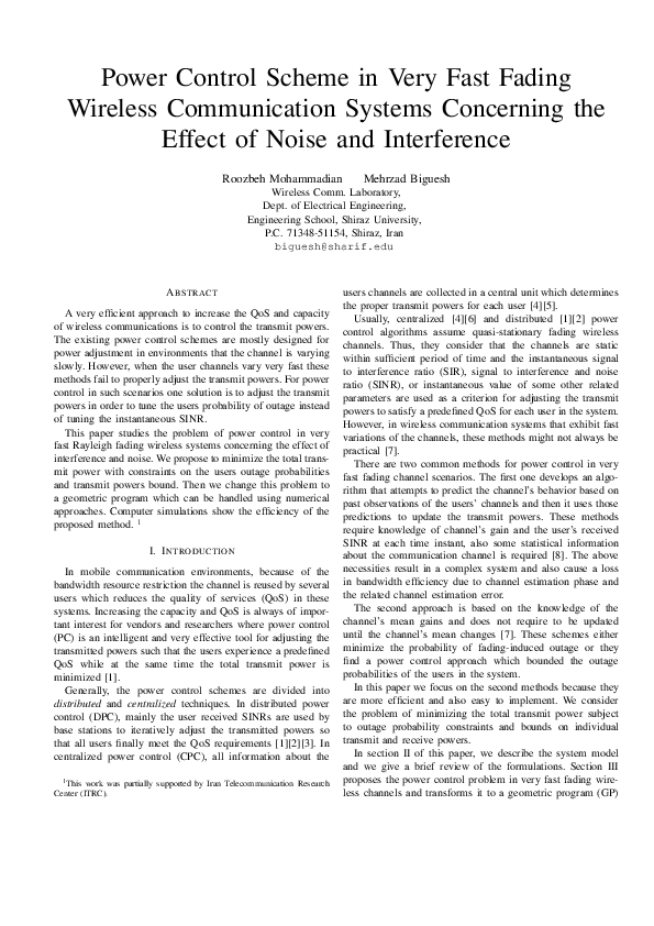ln[gi (y)] ≤ 0, ln[fi (y)] = 0, (13) i = 1, · · · , m i = 1, · · · , p 5.5 1.25 5 1.2 4.5 1.15 transmitter 2 transmitter 3 1.1 4 Optimal transmit power Total transmit power transmitter 1 3.5 3 2.5 1.05 1 0.95 0.9 2 0.85 1.5 0.8 1 5 Fig. 1. 10 15 Number of iterations 20 25 Learning curve for the transmit powers. which is called the convex form of the GP and is a convex optimization problem. This is because the objective and inequality constraint functions are all convex and equality constraint functions are affine. Note that the convex form of a GP problem can be solved globally with great efficiency, using recently developed interior-point methods [10]. V. C OMPUTER SIMULATIONS For computer simulations, we consider a cellular wireless network with M = 3 transmitters and receivers. The path gain, Gii between the ith transmitter/receiver pair is assumed to be 1 and gains Gik (for i 6= k) are independent random variables with uniform distribution over 0.001 and 0.004. Maximum allowed outage probabilities are Oimax = 0.01 for i = 1, 2, 3. We select Pimax = 3 and Pth = 10−3 . The δ1 and δ2 (the coefficients for upper and lower bounds of approximation) are set to 0.9 and 1.1, respectively. The CDMA de-spreading gains are assumed to be θii = 128 and θik = 1 for i 6= k and the error tolerance is ǫ = 10−5 . In the first scenario, we assume γth = 5dB and σ 2 = 0.5. The program is executed for 100 times with random initial feasible powers Pi uniformly distributed between 0.5 and 2. Over the entire set of experiments our algorithm converged to a unique optimal set of transmit powers. Fig. 1 shows the learning curves for the elements of P over this simulation experiments. Here, the average number of iterations for convergence of the algorithm is approximately 12. In the second simulation, we have used σ 2 = 1. In this case, Fig. 2 shows the required transmit powers for the users of our scenario as a function of γth for one run of the simulation. Our other simulations show that the solution of our approximate method is in excellent match with the exact solution found using exhaustive search. VI. C ONCLUSION Power control is a very efficient scheme to enhance the capacity and QoS of mobile communication systems. Evidently, in fast time-varying environments the power control algorithms designed for environments with quasi-stationary channels do 0.75 0 2 Fig. 2. 4 6 8 10 12 Threshold SINR(dB) 14 16 18 20 Required transmit power as a function of γth . not work properly. We proposed a new centralized power control problem for mobile communication systems with fast Rayleigh fading channels. The proposed power control problem minimizes the total transmit power with constrains on outage probability for each user in the system and with constraints on individual transmit and received signal powers. The proposed problem was casted to a standard geometric problem which is solvable using efficient numerical methods. Our computer simulations show that, this new algorithm performs quite well, and it seems to provide a global optimal power vector, independent of the initial point of search in geometric programming. R EFERENCES [1] J. Zander, “Distributed cochannel interference control in cellular radio systems,” IEEE Trans. Veh. Technol., vol. 41, no. 3, pp. 305-311, Aug. 1992. [2] G. J. Foschini and Z. Miljanic, “Distributed autonomous wireless channel assignment algorithm with power control,” IEEE Trans. Veh. Technol., vol. 44, no. 3, pp. 420-429, Aug. 1995. [3] M. Biguesh, A. B. Gershman, and A. Czylwick, “An improved distributed downlink power control in the presence of erroneous user SINR reports,” in Proc. IEEE Vehicular Technology Conference (VTC), Milan, Italy, May 2004. [4] S. A. Grandhi, R. Vijayan and D. J. Goodman, “Centralized power control in cellular radio systems,” IEEE Trans. Veh. Technol., vol. 42, no. 4, Nov. 1993. [5] H. Boche and M. Schubert, “A new approach to power adjustment for spatial covariance based downlink beamforming,” in Proc. IEEE International Conference Acoustics, Speech, and Signal Processing, vol. 5, pp. 29572960, Salt Lake City, Utah, USA, May 2001. [6] H. Alavi and R. Nettleton, “Downstream power control for a spread spectrum cellular mobile radio system,” in Proc. GLOBECOM, pp. 8488, Nov. 1982. [7] S. Kandukuri and S. Boyd, “Optimal power control in interferencelimited fading wireless channels with outage-probability specifications,” IEEE Trans. Wireless Communications, vol. 1, pp. 46-55, Jan. 2002. [8] T. Holliday, A. Goldsmith and P. Glynn “Distributed power control for time varying wireless networks: optimality and convergence ,”Proceedings: Allerton Conference on Communications, Control, and Computing, Monticello, IL, pp. 1024-1033, Oct. 2003. [9] S. Boyd, S. J. Kim, L. Vandenberghe and B. Hassibi, “A toturial on geometric programming,” Stanford University EE Technical Report, 2005. [10] S. Boyd and L. Vandenberghe, Convex Optimization, Cambridge University Press, 2004.