Engineering Geology 123 (2011) 225–234 Contents lists available at SciVerse ScienceDirect Engineering Geology journal homepage: www.elsevier.com/locate/enggeo Landslide susceptibility assessment using SVM machine learning algorithm Miloš Marjanović a,⁎, Miloš Kovačević b, 1, Branislav Bajat b, 2, Vít Voženílek a, 3 a b Faculty of Science, Palacky University, Tř. Svobody 26, 77146 Olomouc, Czech Republic Faculty of Civil Engineering, University of Belgrade, Bulevar kralja Aleksandra 73, 11000 Belgrade, Serbia a r t i c l e i n f o Article history: Received 28 August 2010 Received in revised form 24 August 2011 Accepted 4 September 2011 Available online 19 September 2011 Keywords: Landslide susceptibility Support Vector Machines Decision Tree Logistic Regression Analytical Hierarchy Process Classification a b s t r a c t This paper introduces the current machine learning approach to solving spatial modeling problems in the domain of landslide susceptibility assessment. The latter is introduced as a classification problem, having multiple (geological, morphological, environmental etc.) attributes and one referent landslide inventory map from which to devise the classification rules. Three different machine learning algorithms were compared: Support Vector Machines, Decision Trees and Logistic Regression. A specific area of the Fruška Gora Mountain (Serbia) was selected to perform the entire modeling procedure, from attribute and referent data preparation/ processing, through the classifiers' implementation to the evaluation, carried out in terms of the model's performance and agreement with the referent data. The experiments showed that Support Vector Machines outperformed the other proposed methods, and hence this algorithm was selected as the model of choice to be compared with a common knowledge-driven method – the Analytical Hierarchy Process – to create a landslide susceptibility map of the relevant area. The SVM classifier outperformed the AHP approach in all evaluation metrics (κ index, area under ROC curve and false positive rate in stable ground class). © 2011 Elsevier B.V. All rights reserved. 1. Introduction Natural hazards adversely affect humanity on different scales. They occur at varying intervals and are of differing duration. They have both social and economic consequences. Strategies for their management ought to deal with not only existing hotspots (Nadim et al., 2006), but also with potential new ones, by predicting their behavior, volume and severity prior to their occurrence. Of these, landslides, or mass movements of land are considered in this paper. Even though they are often underestimated when compared to the effects of related phenomena such as floods, earthquakes, volcanoes, storms and so forth, landslides seem to be among the top seven natural hazards (Aleotti and Chowdhury, 1999; Nadim et al., 2006). Lately, due to the worldwide growing needs of urbanization and land exploitation in unstable climatic conditions, there has been a significant growth in interest in landslide assessment topics, resulting in frequent multidisciplinary case studies and raising the number of scholars per investigation (Gokceoglu and Sezer, 2009). Landslide susceptibility (Varnes, 1984) is broadly confused with landslide hazard, mainly because real hazard assessment appears to be feasible only for limited areas with excellent data coverage ⁎ Corresponding author. Tel.: + 420 585 634 525; fax: + 420 585 225 737. E-mail addresses: milos.marjanovic01@upol.cz (M. Marjanović), milos@grf.bg.ac.rs (M. Kovačević), bajat@grf.bg.ac.rs (B. Bajat), vit.vozenilek@upol.cz (V. Voženílek). 1 Tel.: + 381 11 3218 589. 2 Tel.: + 381 11 3218 579. 3 Tel.: + 420 585 634 513. 0013-7952/$ – see front matter © 2011 Elsevier B.V. All rights reserved. doi:10.1016/j.enggeo.2011.09.006 (Carrara and Pike, 2008). Nevertheless, the entire range of problems is encountered in the landslide assessment framework, including the quality of the input data, lack of historical evidence on landslide occurrences, absence of triggering event analyses and model evaluation, as well as interpretational difficulties on the scientist–decision maker basis (Carrara and Pike, 2008). In recent years a great variety of spatial data has become publicly accessible in digital form, thus enabling the utilization of new datadriven methods in processing and analyses. The emerging field of computer science which studies the algorithms that learn from the available data in order to perform processing tasks such as classification, prediction or clustering is called machine learning (Mitchell, 1997). The basic concepts of machine learning and its applications in spatially distributed data are given in Kanevski et al. (2009). Landslide susceptibility has been illustrated in versatile techniques in various case studies, yielding more or less reliable results (Chacón et al., 2006), depending on the complexity of the terrain and the suitability of the approach, (Bonham-Carter, 1994). The central ideas of all those studies imply the processing of the input parameters into a single output model through the various weighting, calculating and interpolating methods i.e. expert-based (heuristic) approach, deterministic (physically-based) models and machine learning techniques. Very detailed reviews of such examples can be found in Chacón et al. (2006), Aleotti and Chowdhury (1999), Brenning (2005, 2008), Guzzetti et al. (1999). All those attempts came to a common conclusion; that the problematic dealt with in the scope of landslide assessment tends to be non-linear, due to the complexity of the geological environment, as well as the factors 226 M. Marjanović et al. / Engineering Geology 123 (2011) 225–234 relating to the triggering itself (storms, earthquakes, erosion, human influence, etc.). Most of those studies also signify the inevitable presence of spatial autocorrelation in every input attribute, which, if not taken into consideration could lead to erroneous results (Brenning, 2005, 2008). This research compares three different learning methods in the task of landslide susceptibility mapping. After analyses were conducted over the case study area, a Support Vector Machines method was chosen to be compared with the common knowledge-driven method — the Analytical Hierarchy Process. One of the foci was to examine the stability of the machine learning model in relation to the size of the training set, as well as the generalization capabilities of induced models, in order to demonstrate that fair susceptibility interpretation is feasible from sparse (or “a low number of”) inputs, as indicated in some earlier works (Yao et al., 2008). A successful solution for susceptibility mapping with optimized algorithms as proposed for this particular case study could be designed to be used with adjacent terrains in order to automatically produce the satisfactory landslide susceptibility map. The proposed approach could serve different scales and levels of detail of Urban Planning or Disaster Management affairs, in order to prevent or reduce the landslide-related risk. The structure of the paper is as follows: Section 2 defines the scope of the research. Section 3 gives an insight into related works concerning the usage of machine learning methods in landslide assessment. A brief description of the theoretical foundations of the Support Vector Machines approach used for landslide classification and the selected knowledge-driven method is given in Section 4. In addition, it contains a description of the proposed model evaluation metrics. Section 5 provides details of the experiments performed in the case study area in northern Serbia. It describes the testing protocol and the analysis of the experimental results. Section 6 concludes the paper. 2. Problem formulation The main objective of this research is to examine the possibility of automating the process of landslide susceptibility mapping by using machine learning techniques. The desired automated procedure assumes that after the initial acquisition of the necessary spatial data, an expert is presented with a (possibly small) representative region of the whole terrain. Such a scenario assumes a supervised learning approach in which the expert performs mapping in the representative region and the map subsequently produced is used for training the machine which would perform the mapping task in the rest of the area. Three different learning methods (Support Vector Machines — SVM, Decision Trees — DT and Logistic Regression — LR) were tested for their ability to perform the mapping task on a specified terrain. After the selection of the method which performed the best, it is compared to the common knowledge-driven approach (Analytical Hierarchy Process — AHP). Assuming that the input data (terrain attributes and referent landslide map) are organized as raster sets, where each grid element (pixel) represents a data instance at a certain point of the terrain, the proposed approach leads to a classification task, which places each pixel from the raster map into an appropriate landslide category using the terrain attributes associated with that pixel. In this research we were partly faced with the problem of determining the number of training examples used to teach the machine — the number of pixels processed by the expert. A good approach is to build a sufficiently accurate model with a smaller number of training examples, thus leading to a reduced expert engagement. We can briefly formulate the landslide classification problem. Let P = {x|x ∈ R n} be the set of all possible pixels extracted from the raster representation of a given terrain. Each pixel is represented as an n-dimensional real vector where coordinate xi represents the value of the i-th terrain attribute associated with the pixel x. Further, let C = {c1, c2, …, cl} be the set of l disjunctive, predefined landslide susceptibility classes (as opposed to many other papers in the field, in this case there are three classes of interest: stable ground, dormant and active landslides). A function fc : P → C is called a classification if for each xi ∈ P it holds that fc(xi) = cj whenever a pixel xi belongs to the landslide susceptibility class cj. In practice, for a given terrain, one has a limited set of m-labeled examples (xi, ci),xi ∈ Rn, ci ∈ C, i = 1,…, m (m being a reasonably small amount of instances). Labeled examples form a training set for the classification problem at hand. The machine learning approach tries to find a function f˜c , which is a good approximation of a real, unknown function fc , using only the examples from the training set and a specific learning method. In Section 4, a brief theoretical background of Support Vector Machines and the Analytical Hierarchy Process is given. Decision trees and Logistic Regression are explained in (Quinlan, 1993) and (Hosmer and Lemeshow, 2000) respectively. All classification experiments were performed within an open-source package, Weka 3.6 (Hall et al., 2009). 3. Related work Pioneering the application of SVM in landslide susceptibility Yao and Dai (2006) and Yao et al. (2008) compared single-class to twoclass (binary) SVM in the Hong Kong area. The authors demonstrated how the latter provided better conditions for algorithm training and testing, since it is clearly favorable to know where the landslides exist and where they do not. The Study by Yuan and Zhang (2006) regarded a specific type of landslide phenomena, the debris flows, by comparing SVM and the fuzzy approach. Since it outperformed the fuzzy method in the testing mode, SVM was considered appropriate and more convenient for this kind of assessment in the area of interest (Yunnan Province, China). As with SVM, Decision Trees are rather novel in the landslide analysis framework, but some successful studies have taken place recently (Saito et al., 2009; Yeon et al., 2010). Their potential is more related to Expert Systems design, since most of the DT techniques give an insight into particular conditions that are potentially correlated with landslide occurrences (decomposing the tree to a congregation of rules gives an insight into the attribute–landslide relationship). Logistic Regression on the other hand, has a longer tradition in natural hazard assessment, and landslide susceptibility is no exception. It has been proven successful in numerous case studies (Falaschi et al., 2009; Bai et al., 2010; Kanungo et al., 2006), but lately it has been broadly challenged by other machine learning approaches. Individual case studies point only to the specific merits or shortcomings of the models, so to illustrate the true value of the SVM, LR, DT or any other method, comparative studies are mandatory (Carrara and Pike, 2008). Few such contributions have been made. The first study we will mention concerned a case study from the Ecuadorian Andes (Brenning, 2005) which employed Logistic Regression, Decision Trees and SVM. The author emphasized the necessity of thorough input data preparation, and pointed to the overoptimistic expectations for the machine learning techniques (when training on one and testing on adjacent area, the result yields much poorer performance). Finally, very recent comparative research (Yilmaz, 2009) appeared in the field, with a very complete perspective on the landslide assessment methodology. Various modeling methods have been considered and compared, including ANN and SVM techniques. The study shows that several methods are very precise and efficient. 4. Methods 4.1. Support Vector Machines Originally, SVM is a binary classifier (instances could be classified to only one of the two classes), but one can easily transform n-class problems into the sequence of n (one-versus-all) or n(n − 1) / 2 (one-versus-one) binary classification tasks (Belousov et al., 2002). M. Marjanović et al. / Engineering Geology 123 (2011) 225–234 The basic variant of the algorithm attempts to generate a separating hyper-plane in the original space of n coordinates (xi parameters in vector x) between the points of two distinct classes. 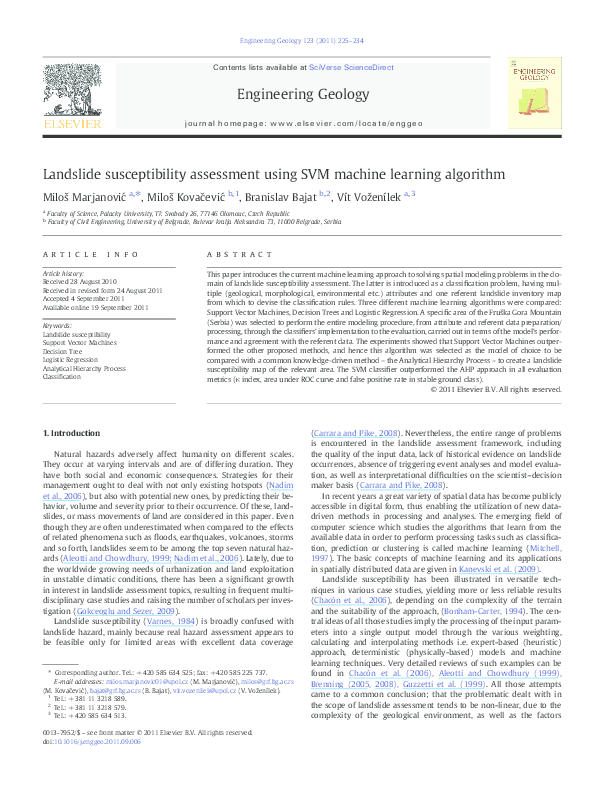The SVM differs from other separating hyper-plane approaches in the way the hyper-plane is constructed from the training set points (Fig. 1a). The algorithm seeks a maximum margin of separation between the classes (M2 N M1 in Fig. 1a) and constructs a classification hyperplane in the middle of the maximum margin (f(x) in Fig. 1a). If a point x ∈ R n is above the hyper-plane, it is classified as + 1 (squares in Fig. 1a), otherwise it is −1 (circles in Fig. 1a). The classification function is therefore given with Eq. (1) in which y represents the class label, w and b are the parameters of the hyper-plane and sgn denotes the sign function. It has been proven that a maximum-margin classifier has the best generalization capabilities on unseen data when compared to other possible separating hyper-plane solutions (Vapnik, 1995). n ! y ¼ sgnðf ðxÞÞ ¼ sgn ∑ wi xi þ b i¼1 ¼ sgnðw · x þ bÞ ð1Þ 227 An interesting property of the optimal hyper-plane is that many αi are equal to zero, and hence the solution (2) depends only on the subset of training points called support vectors — these are the points that contain sufficient information about classes. In order to cope with the non-linearity of the classification problem, the SVM approach goes a step further. One can define the mapping of examples to a so-called feature space of very high dimension: ϕ : Rn →Rd ; n≪d i.e. x→ϕðxÞ. The basic idea of this mapping into high dimensional space is to transform the non-linear case into a linear one as illustrated in Fig. 1c,d (where R 1 inseparable case becomes separable in R 2) and then to use the linear algorithm that has already been mentioned. In such space the dot-product from Eq. (2) transforms into ϕðxi Þ·ϕðxÞ. Certain classes of functions called kernels exist for which kðx; yÞ ¼ ϕðxÞ·ϕðyÞ holds, meaning that they represent dot-products in some high dimensional spaces (feature spaces), yet could be easily computed into the original space. The most popular kernels used in SVM classification tasks are polynomial kernels and Radial Basis Function (RBF), also called Gaussian kernels. By using some of these kernels Eq. (2) becomes: m Real classification datasets are noisy and linearly non-separable. Hence, the algorithm for finding f(x) allows some points to be on the wrong side of the hyper-plane (Fig. 1b). The soft-margin classifier is therefore constructed to balance between the generalization capacity (wide margin width) and the empirical error (sum of training errors ek) of the classification model. If one allows many erroneous points, the model becomes less complex but cannot capture the class distributions (poor generalization capacity). In addition, if there are very few errors, the model becomes very complex and once again its generalization capacity is small. SVM training introduces a parameter C N 0 which controls this trade-off (larger values of C produce more complex models). The solution for optimal hyper-plane weightsmw can be expressed as a linear combination of training points w ¼ ∑ αi yi xi ; i ¼ 1; …m . i¼1 Eq. (1) now becomes: m f ðxÞ ¼ sgn ∑ αi yi ðxi · xÞ þ b i¼1 ð2Þ f ðxÞ ¼ sgn ∑ αi yi kðxi ; xÞ þ b ð3Þ i¼1 In this paper a Gaussian kernel Eq. (4) was used to cope with the non-linear nature of the problem. It initially gave encouraging results and was included in the further optimization procedure described in Section 5.3.   2 kðx; yÞ ¼ exp −γjjx−yjj ð4Þ In order to achieve the numerical stability of the SVM learning method, we scaled both training and test sets in all our experiments by using linear transformation of inputs (each attribute value is divided by the corresponding maximum value from the training set). These sets were used for other compared methods, too. A more detailed review of SVM algorithm for pattern classification can be found in Burges (1998) and Kecman (2005). Kernel methods are thoroughly described in Cristiani and Shawe-Taylor (2000). Fig. 1. a) Maximum-margin classifier f(x) separating circles from squares in R2; b) Soft-margin classifier allows some points to be misclassified; c) Linearly inseparable case in R1; d) Mapping original input space into feature space of higher dimension (R2). Classes become linearly separable after the mapping. 228 M. Marjanović et al. / Engineering Geology 123 (2011) 225–234 4.2. Analytical Hierarchy Process One widespread knowledge-driven method was proposed, in order to challenge the SVM-driven solution. It involved heuristic multi-criteria analyses, which required weighting and a ranging of input data in a somewhat subjective but fast and efficient manner. Attributes Ai were first reclassified by natural breaks cutoffs and ranged to appropriate values (0–100). Each input attribute was weighted (Wi) according to its importance for the landsliding process, as judged by several studies (Komac, 2006; Voženílek, 2000). Criteria quantification was performed through the Analytical Hierarchy Process (AHP) (Saaty, 1980) and final weights Wi were embedded into an additive function L, as indicated in Eq. (5), in a GIS environment, retrieving the continual AHP-driven raster model of landslide susceptibility. In order to evaluate its performance against the referent map, this result needed to be reclassified in the same fashion as the reference. For this purpose the most convenient method was a 3-fold logarithmic cutoffs selection, which delivered classification intervals in respect of the referent map. 12 L ¼ ∑ Wi Ai ð5Þ i¼1 4.3. Model evaluation metrics The quality of classification could be simply estimated as the relation between correctly and incorrectly classified instances, but the problem of proper evaluation becomes more complex (Frattini et al., 2010), and requires more sophisticated solutions, and in this paper two such solutions were considered. The first involved Receiver Operating Characteristics (ROC), which is a cut-off independent performance estimator (Fielding and Bell, 1997). It involves the inspection of False Positives — FP (misclassified landslide instances — classifier labels pixel as class A, expert disagrees) and False Negatives — FN (misclassified non-landslide instances — expert labels pixel as A, classifier disagrees) inspection. ROC values are created by plotting the cumulative rates of FP (sensitivity) versus rates of FN (specificity) for every model, resulting in a set of ROC curves. The performance is evaluated by the Area Under the Curve (AUC) relative to the entire plot area, so that an AUC equal to 1 has the best performance, while an AUC as low as 0.5 results in a very poor performance (Frattini et al., 2010). The second method concerns the agreement coefficient, also called the κ-index, which represents the measure of agreement between compared entities, rather than the measure of classification quality (Landis and Koch, 1977). It is quite convenient for the map comparisons if an equal number of classes applies (Bonham-Carter, 1994), which was the case in this research. The idea of κ is to remove the effect of the random agreement between the two experts (here, between classifier-driven and AHP-driven maps on the one hand and referent landslide map on the other). The Obtained index ranges from − 1 for the complete absence of agreement to +1 for the absolute agreement. Zero values suggest that the agreement is no different from the original odds of having coinciding classes between two maps. Based on Landis and Koch (1977) the κ-index, values falling within a range of 0.61–0.81 are categorized as substantial, and values higher than 0.81 are considered as nearly perfect. 5. Experiments 5.1. Case study area The study area encompasses the NW slopes of the Fruška Gora Mountain, in the vicinity of Novi Sad, Serbia (Fig. 2). The site (N 45°09′20″, E 19°32′34″–N 45°12′25″, E 19°37′46″) spreads over approximately 100 km 2 of hilly landscape, but with interesting dynamics and an abundance of landslide occurrences. The geological setting of the entire mountain reveals a zonal composition caused by the complex E–W trended horst-anticline. The typical succession (Pavlović et al., 2005) starts with Paleozoic metamorphic rocks in the anticline base, encompassing the ground above 300 m and underlying all younger formations. Triassic basal sediments (conglomerates and sandstones gradually shifting toward the limestones) imply localized subsidence in the relief at the time of the basin's formation. The closing of that basin during the Jurassic– Cretaceous, left typical oceanic crust evidence (ultra-mafic unit) as well as gulf limestone sequences. The Tertiary is chiefly represented by marine sediments, gaining more carbonate components as the basin turned more limnic during the late Neogene. The most widespread Quaternary unit is loess, which covers the lower landscape toward the Danube on the north. In geotechnical practice, it is believed that the superficial dynamics directly depend on geological background, meaning that the rocks' behavior under agencies of different processes yields diverse geodynamic outcomes (Janjić, 1962). Geomorphological evidence supports these expectations for our relatively small study area (Fig. 2), where slope stability can be generalized into several scenarios (Fig. 3). The higher ground, chiefly composed of metamorphic rocks, is mostly shaped by fluvial and slope processes, where shallow valleys and gullies are cut into the bedrock, forming a dense drainage pattern. Because they are not severely tectonized, moderately inclined and mostly vegetated, the dominating slope processes on the flanks of these rocky valleys are screes, minor rockfalls and minor shallow landslides (Fig. 3a). The middle plateau (Fig. 2) is formed of carbonate and clastic rocks and has insufficient thickness to develop karstification, so the fluvial forms still predominate. However, the slope processes are better developed, especially in Miocene–Pliocene marlstones and clays, where deep-seated landslides (slips up to 10– 20 m in depth) are hosted (Fig. 3b), particularly on the steeper slopes (slope N 20°). The morphology of the lowest ground that flattens toward the north is governed by the fluvial dynamics of the Danube. It is represented by sequences of river terraces, inundation plains and the alluvial fans of smaller tributaries. This is where the loess formations are facing the river as relatively steep cliffs. In spite of the general stability of loess, landslides on the cliff faces are quite common along the riverbank. The latter is caused by surges of groundwater that locally communicate through the bedrock (Fig. 3c), keeping the loess units in unfavorable conditions (saturation and suffosion). Moreover, loess usually consists of overlaying clays and marls that are likely hosting the fossil landslides and seizing the loess slabs above them (Fig. 3c). It seems apparent that the instabilities are generally driven by geological, geomorphometric, and environmental attributes (such as lithology, elevation, slope angle, land cover and so forth) which was further elaborated in this study. 5.2. Input datasets Being a non-linear classification problem, landslide susceptibility investigation fits the description of the problematic addressed in previous passages. It has already been indicated that conventional techniques for this type of research involve the use of a modeling method with an input dataset of important terrain attributes, which are being selected according to the data availability and the significance of data in relation to the problem at question. Although a majority of researchers use all available data and measure their statistical dependence against landslide occurrences prior to their implementation, it is suggested that the input attributes are chosen more cautiously, due to their temporal durability and scale constrictions. Namely, it is considered that in landslide susceptibility analysis, M. Marjanović et al. / Engineering Geology 123 (2011) 225–234 229 Fig. 2. Geographical location (GK grid, zone 7) and geological setting of the study area (Fruška Gora Mountain, Serbia). Legend: Pz — Paleozoic low grade metamorphic rocks (phyllite, greenschists), Se — ultramafic rocks (serpentinite of Jurassic age), M1 — lower Miocene limestone, marlstone, sandstone and sand, M2 — upper Miocene organic limestone and marl, Pl — Pliocene marl and clay, l — loess, dl — diluvium cover, a′ — terrace sediments (gravel and sand), a — alluvium deposits (gravel and sand). constant variables (regarding the time scale of the landsliding process) should be preferred, meaning that attributes such as land use, climate data, pore-water pressure data and others that have distinct annual or even diurnal variations, should be used with caution (Ohlemacher, 2007). Thematic layers were acquired from different resources, entailing different levels of generalization and different scales, and subsequently compiled to an optimal 30 m raster cell resolution. Their assemblage represents our input dataset, first prepared by ArcGIS and SAGA GIS packages (Böhner et al., 2006) to be finally converted to ASCII files (to commute with machine learning software in absence of fully integrated modules). The descriptions of used input data, their spatial resolution and sources are given in Table 1. The general statistics for all attribute layers and information gain ranking (Quinlan, 1993) based on overall terrain data are shown in Table 2. The information gain ranking bears out the usage of all three different sources of input data: topographic attributes — DEM, lithology — geological map, and NDVI — LANDSAT imagery. Fig. 3. Schematic cross-sections of typical slope instability scenarios over the study area: a) shallow landslide in the diluvium cover on the valley side, b) deep-seated landslide in clay, c) landslide in saturated loess (groundwater percolates from the porous bedrock toward loess as clay layer wedges down) d) loess slabs seized by reactivated fossil landslide. Legend: 1 — phylitte/greenschist (Pz), 2 — limestone (calcarenite) and marlstone (M1), 3 — gravelly sand (M1), 4 — marl (M2), 5 — sandy clay (Pl), 6 — loess with loam layers (Q), 7 — diluvium cover (Q); vertical and horizontal scale are the same. 230 M. Marjanović et al. / Engineering Geology 123 (2011) 225–234 Table 1 Raster thematic maps of input dataset. Spatial data attributes (notation) Source, scale/resolution Short description Elevation (A1) Slope (A2) Aspect (A3) Slope length (A4) Topographic wetness index (A5) Plan curvature (A6) Profile curvature (A7) Distance from stream (A8) Lithology⁎ (A9) Distance from fault (A10) Distance from geo-boundary (A11) NDVI (A12) Topo-maps, 1:25,000 DEM, 30 m DEM, 30 m DEM, 30 m DEM, 30 m DEM, 30 m DEM, 30 m DEM, 30 m Geo-map, 1:50,000 Geo-map, 1:50,000 Geo-map, 1:50,000 Landsat image, 30 m DEM of the terrain surface Angle of the slope inclination Exposition of the slope Length factor of the slope Ratio of contributing area a and tg (slope) Index of concavity parallel to the slope Index of concavity perpendicular to slope Buffer of drainage network Rock units Buffer of structures Buffer of boundaries between rock units Interpretation of vegetation, water bodies and bare soil, based on NDVI ⁎ To avoid subjective quantification of nominal classes, this attribute was actually isolated into n dummy variables, giving n-bit class codes for class units, where n is the number of classes in the attribute (e.g. limestone — class 3 in lithology is coded as 00100000000). Topographic data were obtained from the standard topographic maps of Serbia at the scale 1:25,000, where contour lines generated from a conventional photogrammetric restitution are given, with the equidistance of 10 m. For the generation of the Digital Elevation Model (DEM), these contour lines were first digitized, then decomposed to point data, interpolated by triangulation, and converted to raster format with 30 m cell resolution. Even though topographic maps with a given scale are suitable for DEM's productions with denser resolutions (Carrara et al., 1997), a DEM resolution of 30 m was chosen for two reasons; as the proper DEM resolution for regional landslide modeling (Gruber et al., 2009) and as the adequate support grid size compatible with other data sources used in this study, such as a geological map to the scale 1:50,000 and 30 m Landsat imagery. All DEM-related geomorphometric and hydrological thematic maps kept the same (30 m) resolution. Within the framework of The Vojvodina Province governmental project on Geological conditions of rational exploitation of the Fruška Gora Mountain area, completed in 2005 by the expert team of the Faculty of Mining and Geology of Belgrade University, a set of different thematic maps was generated for the entire mountain area, including geological, geomorphological, photogeological, pedological, seismological etc. In this research some of those resources were utilized thanks to the courtesy of the Faculty of Mining and Geology. Geological data were obtained from the above mentioned digital Geological map at 1:50,000 scale. This map was compiled from a terrain Geological map at 1:25,000 and the Basic Geological map of Serbia at the scale of 1:100,000. Since it is not formational but chronostratigraphic, the map was simplified even further for the purpose of our case study (it contained many rock units of similar physical properties, which could be a drawback for the analysis, so the simplification was governed toward formational criteria). Therefore, the generalization to a raster map with 30 m resolution was justifiable. The photogeological map (1:50,000) represents the coupled geomorphological and structural map, that stresses the forms of the most current geological processes at play. It is compiled by adopting basic geomorphological units and appending the heuristic (Remotesensing-based) structural and stability interpretation. The latter was performed as an expert-based analysis of 30 m Landsat TM imagery and auxiliary derivates (enhancements and processed images), as well as orthorectified aerial photographs at 1:33,000 scale. In this research, the emphasis was on utilizing the stability analysis, so only that part was extracted from the photogeological map. In this manner, the Landslide reference raster map at 30 m resolution was obtained (landslide inventory). This map reveals the stability of the landscape by distinguishing several classes of landsliding processes, chiefly dormant and active landslide scarps (Fig. 4a). According to the adopted classification (Varnes, 1984), landslide instances fell into the category of rotational and translational type of slides, while other, minor occurrences of flows and falls were not taken into consideration. The map depicted the distribution of classes into the following categories: 3.6% active slides, 5.6% dormant slides and the remaining 90.8% conditionally stable ground. Environmental information particularly regarded the vegetation cover, due to possible remediation that some vegetation types can provide for shallow landslidng (the influence of root cohesion, moisture retention). There are numerous vegetation indices proposed, to estimate biomass and delineate different types of vegetation apart from bare soil, rock, wetlands and artificial surfaces (Glenn et al., 2008). After experimenting with several indices we acknowledged the Normalized Difference Vegetation Index (NDVI), which basically delimits the chlorophyll spectra. For this purpose, 30 m Landsat TM Table 2 General statistics of attribute layers. Terrain attribute (unit) Maximum value Minimum value Mean value Standard deviation Info. gain ranking Elevation (m) Slope (°) Aspect (°) Slope length (m) Topographic wetness index Plan curvature Profile curvature Distance from stream (m) Lithology⁎ Distance from fault (m) Distance from geo-boundary (m) NDVI 523.19 40.16 359.99 6456.41 22.49 3.3725 4.0607 1225.60 ⁎ 79.83 0.00 − 1.00 0.00 7.56 − 4.0694 − 2.6968 0.00 ⁎ 241.64 11.77 173.26 103.77 11.51 0.0085 0.0089 319.59 ⁎ 94.61 6.62 116.47 152.19 2.83 0.0085 0.4060 224.89 ⁎ 1672.75 1465.09 0.56 0.00 0.00 − 0.75 309.85 306.32 0.17 259.11 295.45 0.21 1 5 10 11 4 9 8 6 2 7 12 3 ⁎ Nominal attribute. 231 M. Marjanović et al. / Engineering Geology 123 (2011) 225–234 Fig. 4. Referent landslide inventory map a) and landslide susceptibility models of the balanced training set experiments: RS-B SVM10% Support Vector Machine model b); RS-B LR10% Logistic Regression model c); RS-B DT10% Decision Tree model d). In our problem setting we performed two groups of experiments concerning the spatial distribution of training and test data: a random training subset uniformly distributed over the whole case study area (RS) and a train-test split derived from two independent, neighboring parts of the whole case study area (NS). The RS group consisted of two different experiments concerning the choice of training points: the first assumed usage of all points in the random sample (A), while the second used a balanced approach in which the number of non-landslide points is equal to the sum of landslide points (B). Both RS-A and RS-B were performed in three different iterations in which a random subset consisted of 5% (6156), 10% (12,313) and 15% (18,496) of points from the whole case study area. In RS-A, sampling instances were selected randomly, but equally spread over the original area, and they contained a referent class proportion similar to the original landslide model (3.6% of active landslides, 5.6% of dormant landslides, and 90.8% of conditionally stable ground). In order to illustrate the RS-A experimenting procedure, we will describe the course of the RS-A (5%) experiment, while the remaining two are completely analog. The negative effects of randomization (poor estimate of model variance) were minimized by creating 20 different random splits, each containing 5% data points for training and 95% for the test set. It is obvious that these splits are spatially overlapping to some degree, but full separation would not be feasible since some values of many attributes would appear only in the test set. Since there is a lack of information in most related papers concerning the adjustment of SVM learning parameters (Brenning, Table 3 Comparison of the models and the referent landslide map (unbalanced training set). Table 4 Comparison of the models and the referent landslide map (balanced training set). satellite images were used, particularly in the visible and nearinfrared bands. 5.3. Experimental results Model κ-index AUC FP0 Model κ-index AUC FP0 SVM5% LR5% DT5% SVM10% LR10% DT10% SVM15% LR15% DT15% 0.57 0.08 0.42 0.67 0.08 0.42 0.73 0.06 0.54 0.79 0.86 0.76 0.82 0.86 0.76 0.84 0.86 0.80 0.4 0.94 0.56 0.32 0.94 0.56 0.32 0.96 0.43 SVM5% LR5% DT5% SVM10% LR10% DT10% SVM15% LR15% DT15% 0.38 0.25 0.28 0.42 0.25 0.32 0.43 0.23 0.34 0.85 0.85 0.82 0.89 0.85 0.82 0.90 0.86 0.85 0.11 0.23 0.18 0.08 0.24 0.17 0.06 0.20 0.16 232 M. Marjanović et al. / Engineering Geology 123 (2011) 225–234 Table 5 AHP-driven weights Wi of input attributes Ai in respect with Eq. (5). Ai A1 A2 A3 A4 A5 A6 A7 A8 A9 A10 A11 A12 Wi (%) 16.9 19.9 3.3 3.4 8.0 2.0 1.2 6.0 21.8 1.0 5.4 11.1 *Attribute indexes i are given in the same order as in Tables 1 and 2. 2005; Yilmaz, 2009), a procedure of their estimation was conducted. The parameter estimation focused on the penalty factor C and Gaussian kernel width γ. Parameters C and γ took many different values (C = {1, 10, 100, 1000, 10,000} and γ = {0.1, 0.5, 1, 2, 4}). For each combination of (C, γ) a 10-fold cross-validation procedure was performed on a particular training set and the evaluation measures (κindex and AUC) were averaged and recorded for each combination of (C, γ). The results showed that in all 20 splits of the RS-A (5%) experiment, optimal C and γ were the same (100, 4). These values turned optimal for the RS-A (10% and 15%) experiments as well. Given the optimal parameters, the SVM classifier was trained over the entire particular training set and tested over the related test set. The evaluation measures included κ-index, AUC and the false positives rate for non-landslide class (FP0). The above procedure was repeated 20 times for each train-test split and the final measures for the experiment were averaged over all 20 splits. The same evaluation procedure was repeated for DT and LR and the results are given in Table 3. When the number of training points increases, the SVM and DT improve their performance on the κ-index and AUC, while the LR performance remains the same. Concerning the κ-index, the SVM significantly outperformed other models, followed by the DT and LR respectively (very low κ-index for LR). The LR yielded the best AUC when compared to the other two methods, but the SVM came close to the LR when the number of training points increased (0.84 for the SVM compared to 0.86 for the LR). Such a big discrepancy between the κ-index and the AUC in the case of the LR can be explained by understanding that in the non-binary classification setting reported, the AUC represents the weighted sum of class AUCs calculated in a standard binary manner (a particular class against all others) where the weights represent class proportions (Fawcett, 2006). Since our dataset is highly unbalanced, favoring the nonlandslide class, we recorded a false positives rate in the dominant class (column three in Table 3). One can see that the LR exhibits extremely high FP0 when compared to other methods. From the risk assessment point of view this finding completely eliminates the LR as a model of choice since one does not want a landslide terrain to be classified as stable ground. Therefore, we decided to perform another set of RS-B experiments, in which each particular training set had a balanced nature (an equal number of stable and non-stable points). In fact, each training set for RS-B is obtained from the corresponding RS-A set by retaining all landslide points and selecting an equal number of stable points that are spatially uniformly distributed over the whole area. In RS-B experiments the testing protocol remained the same and the results obtained are given in Table 4 (the optimal SVM parameters changed to C = 10 and γ = 4). Generally, the ranking of methods remained similar except the SVM exhibited the best performance in both the κ-index and the AUC for all training set sizes. The biggest gain from the balanced sampling was achieved by the LR method where the AUC remained the same, but the κ-index increased due to a significant decrease in FP0. The SVM and DT methods increased their AUC following the trend of decreasing FP0, but their κ-index decreased due to the increase in the number of stable ground points misclassified as landslides. We believe that this property of these models is more desirable in the application of risk assessment. Furthermore, in order to visualize the results, we retrieved the classification model from RS-B (10%) for the split which had its evaluation measures closest to the average values given in Table 4 (shaded rows). This classifier was then applied to the entire original dataset (all 100%), as it was being remapped into susceptibility maps (Fig. 4b,c,d). A visual impression of those maps supplements the figures from Table 5, which are in favor of the SVM over the DT and LR models. The RS-B SVM map in particular, (Fig. 4b) is the most realistic in following trends of landslide scarps distribution as depicted by the expert (Fig. 4a), while the other two models somewhat disperse either of two landslide classes (active and dormant landslides). It could therefore be speculated that some further generalization (post-processing filtering) could improve the mapping accuracy to some extent. In the NS experiment (Fig. 5b) the area under consideration was divided in two separate, neighboring parts, where the training part occupied approximately one third (nearly 41,000 points) of the whole area (123,134 points). The spatial division was made in order to produce the training set in which all lithological classes will be presented in the training area. From Tables 3 and 4 one can conclude that the SVM is the best performing model and hence it was tested against the AHP method (AHP-driven weights Wi of the input attributes Ai are given in Table 5) on the neighboring area. A final, balanced training set was obtained by keeping all landslide points and an equal number of stable ground points which were uniformly distributed over the training area. The comparison results are given in Table 6 and the generated landslide map is shown in Fig. 5. The proposed SVM approach outperformed the AHP (Fig. 5) in all performance measures but the results were significantly weaker in Fig. 5. AHP landslide susceptibility model a); NS SVM10% model with training area represented as a referent landslide inventory map b). M. Marjanović et al. / Engineering Geology 123 (2011) 225–234 Table 6 Comparison of the models and the referent landslide map for neighboring terrain test set. Model κ-index AUC FP0 AHP SVM10% 0.15 0.17 0.59 0.71 0.73 0.39 comparison to the RS experiments. This finding was expected since the applied classification model was built on a different terrain to the test data, which probably came from a different distribution of input parameters (Brenning, 2005). Finally, we comment on the strengths and weaknesses of the SVM model. Support Vector Machines do not need any feature selection technique as opposed to some other methods such as Decision Trees. This fact enables richer data representation for the input vectors representing terrain pixels. This aspect of the research is left to future work. In addition, since the solution for the SVM separating hyper-plane is found from the convex quadratic programming optimization problem, it is guaranteed that the solution is globally optimal. Therefore, the SVM is a good replacement for Artificial Neural Networks which are usually stuck at local optima and are very difficult to train. On the other hand, the SVM is not an interpretable model like the Decision Trees, and hence could not be rewritten in the form of expert rules. When compared to Logistic Regression, they are much more memory and time consuming during the training phase, but that is probably not of great importance for the task of landslide mapping. 6. Conclusions In this research landslide susceptibility mapping was regarded as a classification task in the input space of DEM, geological and Landsat imagery derived attributes. Terrain pixels (30 m resolution) were classified into three categories: stable ground, dormant and active landslides. Three different learning techniques which learn from expertly labeled data were compared: Support Vector Machines, Logistic Regression and Decision Trees. Two different sampling strategies were conducted in order to create train-test splits for the evaluation of chosen classifiers. The first approach randomly sampled a certain number of terrain pixels from the whole area, retaining the uniform spatial distribution of the selected training points. The second approach divided the whole area into two adjacent parts and then selected from the first part, all landslides points and an equal number of stable ground points to form the training set. While, in the first sampling approach, we tested maximal possibilities of classification models, the second scenario had a very important practical implication — is it possible to automate the creation of landslide susceptibility maps, given the appropriate expert processed data on a neighboring terrain? After conducting experiments based on the first sampling approach, the Support Vector Machines turned to be the model of choice, outperforming other competitors in all evaluation measures (the κ-index and the area under the ROC curve). In addition, the SVM achieved the lowest false positives rate for the stable ground class which is a very important property for risk assessment applications. When comparing the SVM classifier to a common expert-based approach (the Analytical Hierarchy Process) in the mapping task on a neighboring terrain, the former achieved better performance in terms of all evaluation measures than the latter. However, generated maps suggest that much more has to be done to put the automated SVM procedure into operative work. Two possible directions in our future work would be to construct a new set of input features representing terrain pixels, which will include the available information 233 from neighboring points, and to construct a new SVM kernel, other than Gaussian, to incorporate available domain knowledge. Acknowledgments This work was supported by the Czech Science Foundation (Grant of The Czech Science Foundation No. 205/09/079) and the Ministry of Science of the Republic of Serbia (Contract No. III 47014). References Aleotti, P., Chowdhury, R., 1999. Landslide hazard assessment: summary review and new perspectives. Bulletin of Engineering Geology and the Environment 58, 21–44. Bai, S.B., Wang, J., Lü, G.N., Zhou, P.G., Hou, S.S., Xu, S.N., 2010. GIS-based logistic regression for landslide susceptibility mapping of the Zhoungxian segment in the Three Gorges area, China. Geomorphology 115, 23–31. Belousov, A.I., Verzakov, S.A., Von Frese, J., 2002. Applicational aspects of support vector machines. Journal of Chemometrics 16, 482–489. Böhner, J., McCloy, K.R., Strobl, J. (Eds.), 2006. SAGA – Analysis and Modelling Applications, Vol.115. Göttinger Geographische Abhandlungen, Göttinger. 130 pp. Bonham-Carter, G., 1994. Geographic Information System for Geosciences — Modeling with GIS. Pergamon, New York. 398 pp. Brenning, A., 2005. Spatial prediction models for landslide hazards: review, comparison and evaluation. Natural Hazards and Earth System Sciences 5, 853–862. Brenning, A., 2008. Statistical geocomputing combining R and SAGA: the example of landslide susceptibility analysis with generalized additive models. In: Böhner, J., Blaschke, T., Montanarella, L. (Eds.), SAGA – Second Out, vol. 19. Institut für Geographie der Universität, Hamburg, pp. 23–32. Burges, C.J.C., 1998. A tutorial on support vector machines for pattern recognition. Data Mining and Knowledge Discovery 2 (1), 121–167. Carrara, A., Pike, R., 2008. GIS technology and models for assessing landslide hazard and risk. Geomorphology 94, 257–260. Carrara, A., Bitelli, G., Carla, R., 1997. Comparison of techniques for generating digital terrain models from contour lines. International Journal of GIS 11 (5), 451–473. Chacón, J., Irigaray, C., Fernández, T., El Hamdouni, R., 2006. Engineering geology maps: landslides and geographical information systems. Bulletin of Engineering Geology and the Environment 65, 341–411. Cristiani, N., Shawe-Taylor, J., 2000. An Introduction to Support Vector Machines and Other Kernel-Based Learning Methods. Cambridge University Press, Cambridge. 189 pp. Falaschi, F., Giacomelli, F., Fedrici, P.R., Pucinelli, A., Avato, G.D'A., Pochini, A., Ribolini, A., 2009. Logistic regression versus artificial neural networks: landslide susceptibility evaluation in a sample area of the Serchio River valley, Italy. Natural Hazards 50, 551–569. Fawcett, T., 2006. An introduction to ROC analysis. Pattern Recognition Letters 27, 861–874. Fielding, A.H., Bell, J.F., 1997. A review of methods for the assessment of prediction errors in conservation presence/absence models. Environmental Conservation 24, 38–49. Frattini, P., Crosta, G., Carrara, A., 2010. Techniques for evaluating performance of landslide susceptibility models. Engineering Geology 111, 62–72. Glenn, E.P., Huete, A.R., Nagler, P.L., Nelson, S.G., 2008. Relationship between remotelysensed Vegetation Indices, canopy attributes and plant physiological processes: what Vegetation Indices can and cannot tell us about the landscape. Sensors 8, 2136–2160. Gokceoglu, C., Sezer, E., 2009. A statistical assessment on international landslide literature (1945–2008). Landslides 6, 345–351. Gruber, S., Huggel, C., Pike, R., 2009. Modelling mass movements and landslide susceptibility. ch. 23 In: Hengl, T., Reuter, H.I. (Eds.), Geomorphometry: Concepts, Software, Applications. Elsevier, Amsterdam, pp. 527–550. Guzzetti, F., Carrara, A., Cardinali, M., Reichenbach, P., 1999. Landslide hazard evaluation: a review of current techniques and their application in a multi-scale study, Central Italy. Geomorphology 31, 181–216. Hall, M., Frank, E., Holmes, G., Pfahringer, B., Reutemann, P., Witten, I.H., 2009. The WEKA data mining software: an update. SIGKDD Explorations 11 (1), 10–18. Hosmer, D.W., Lemeshow, S., 2000. Applied Logistic Regression. John Wiley & Sons, New York. 375 pp. Janjić, M., 1962. Engineering geology Characteristics of Terrains of National Republic of Serbia (in Serbian). Belgrade, Nučna knjiga. 352 pp. Kanevski, M., Pozdnoukhov, A., Timonin, V., 2009. Machine Learning for Spatial Environmental Data: Theory, Applications and Software. EPFL Press, Lausanne. 368 pp. Kanungo, D.P., Arora, M.K., Sarkar, S., Gupta, R.P., 2006. A comparative study of conventional, ANN black box, fuzzy and combined neural and fuzzy weighting procedures for landslide susceptibility zonation in Darjeeling Himalayas. Engineering Geology 85, 347–366. Kecman, V., 2005. Support vector machines — an introduction. In: Wang, L. (Ed.), Support Vector Machines: Theory and Applications. Springer, Berlin, pp. 1–48. Komac, M., 2006. A landslide susceptibility model using the Analytical Hierarchy Process method and multivariate statistics in perialpine Slovenia. Geomorphology 74, 17–28. Landis, J.R., Koch, G.G., 1977. The measurement of observer agreement for categorical data. Biometrics 33 (1), 159–174. Mitchell, T.M., 1997. Machine Learning. McGraw Hill, New York. 414 pp. 234 M. Marjanović et al. / Engineering Geology 123 (2011) 225–234 Nadim, F., Kjekstad, O., Peduzzi, P., Herold, C., Jaedicke, C., 2006. Global landslide and avalanche hotspots. Landslides 3, 159–173. Ohlemacher, G.C., 2007. Plan curvature and landslide probability in regions dominated by earth flows and earth slides. Engineering Geology 91, 117–134. Pavlović, R., Lokin, P. and Trivić, B., 2005. Geological conditions of racional usage and preservation of the Fruška Gora Mountain area (in Serbian), unpublished, Department for Remote Sensing and Structural Geology, University of Belgrade. Quinlan, J.R., 1993. C4.5: Programs for Machine Learning. Morgan Caufman, San Mateo. 302 pp. Saaty, T.L., 1980. Analytical Hierarchy Process. McGraw-Hill, New York. 287 pp. Saito, H., Nakayama, D., Matsuyama, H., 2009. Comparison of landslide susceptibility based on a decision-tree model and actual landslide occurrence: the Akaishi Mountains, Japan. Geomorphology 109, 108–121. Vapnik, V.N., 1995. The Nature of Statistical Learning Theory. Springer, New York. 316 pp. Varnes, D.J., 1984. Landslide Hazard Zonation: A Review of Principles and Practice. International Association for Engineering Geology, Paris. 63 pp. Voženílek, V., 2000. Landslide modeling for natural risk/hazard assessment with GIS. Acta Universitas Carolinae, Geographica 35, 145–155. Yao, X., Dai, F.C., 2006. Support vector machine modeling of landslide susceptibility using GIS: a case study. 10th IAEG Conference Proceedings, Nottingham, 6–10th September, 2006. IAEG, Nottingham, pp. 1–12. Yao, X., Tham, L.G., Dai, F.C., 2008. Landslide susceptibility mapping based on support vector machine: a case study on natural slopes of Hong Kong, China. Geomorphology 101, 572–582. Yeon, Y.K., Han, J.G., Ryu, K.H., 2010. Landslide susceptibility mapping in Injae, Korea, using a decision tree. Engineering Geology 116, 274–283. Yilmaz, I., 2009. Comparison of landslide susceptibility mapping methodologies for Koyulhisar, Turkey: conditional probability, logistic regression, artificial neural networks, and support vector machine. Environmental Earth 61 (4), 821–836. Yuan, L., Zhang, Y., 2006. Debris flow hazard assessment based on support vector machine. Wuhan University Journal of Natural Sciences 14 (4), 897–900.