Received: 17 March 2024
Revised: 26 June 2024
Accepted: 2 July 2024
DOI: 10.1002/asna.20240034
ORIGINAL ARTICLE
Evaluating a sigmoid dark energy model to explain the
Hubble tension
Camilo Delgado-Correal2
Sergio Torres-Arzayus1
Higuera-G3 Sebastián Rueda-Blanco3
1
Cosmology and Astrophysics
Department, International Center for
Relativistic Astrophysics Network,
Pescara, Italy
2
Physics Department, Francisco José de
Caldas District University of Bogotá,
Bogotá, Colombia
3
Observatorio Astronómico Nacional,
Universidad Nacional de Colombia,
Bogotá, Colombia
Correspondence
Sergio Torres-Arzayus, International
Center for Relativistic Astrophysics
Network, Pescara, Italy.
Email: sergio.torres@icranet.org
Mario-Armando
Abstract
In this study, we analyze Type Ia supernovae (SNe Ia) data sourced from the
Pantheon+ compilation to investigate late-time physics effects influencing the
expansion history, H(z), at redshifts (z < 2). Our focus centers on a time-varying
dark energy (DE) model that introduces a rapid transition in the equation of
state, at a specific redshift, za , from the baseline, wΛ = −1, value to the present
value, w0 . The change in the equation of state is implemented as a transition
in the DE density scale factor driven by a sigmoid function. The constraints
obtained for the DE sigmoid phenomenological parametrization have broad
applicability for dynamic DE models that invoke late-time physics. Our analysis
indicates that the sigmoid model provides a slightly better, though not statistically significant, fit to the SNe Pantheon+ data compared to the standard
Λ cold dark matter (ΛCDM) model. The fit results, assuming a flat geometry
and maintaining Ωm constant at the 2018-Planck value of 0.3153, are as follows: H0 = 73.3+0.2
km s−1 Mpc−1 , w0 = −0.95+0.15
, za = 0.8 ± 0.46. The errors
−0.6
−0.02
represent statistical uncertainties only. The available SN dataset lacks sufficient
statistical power to distinguish between the baseline ΛCDM model and the alternative sigmoid models. A feature of interest offered by the sigmoid model is
that it identifies a specific redshift, za = 0.8, where a potential transition in the
equation of state could have occurred. The sigmoid model does not favor a DE
in the phantom region (w0 < −1). Further constraints to the dynamic DE model
have been obtained using CMB data to compute the distance to the last scattering surface. While the sigmoid DE model does not completely resolve the H0
tension, it offers a transition mechanism that can still play a role alongside other
potential solutions.
KEYWORDS
cosmology, dark energy, Hubble tension, Hubble constant, cosmological parameters
1
I NT RO DU CT ION
The Hubble tension denotes the disparity between the
values of the Hubble constant, H0 , derived from early
Astron. Nachr. 2024;e20240034.
https://doi.org/10.1002/asna.20240034
universe probes, such as the cosmic microwave background (CMB; Bennett et al. 2013) and Baryon Acoustic
Oscillations (BAO) data (Eisenstein 2005), and those measured using the magnitude-redshift relation with data from
www.an-journal.org
© 2024 Wiley-VCH GmbH.
1 of 9
2 of 9
standard candles (late universe) such as Type Ia Supernovae (SNe Ia) using the Cepheid distance scale (Riess
et al. 2022) or calibrated using the tip of the red giant
branch (TRGB) (Freedman et al. 2019). The first signs
of tension between the results from early and late universe probes started showing statistical significance when
comparing the H0 reported by the Hubble Space Telescope
Key Project with H0 = 74.4 ± 2.2 km s−1 Mpc−1 (Freedman et al. 2012), and the Planck mission first release
with H0 = 67.2 ± 1.2 km s−1 Mpc−1 (Planck Collaboration 2014), which is a difference of 3𝜎. For simplicity, the
units of H0 are omitted hereafter (assume km s−1 Mpc−1 ).
It is important to clarify that the Planck results for
H0 are not a direct measurement but a model-dependent
inference, assuming a flat Λ-cold dark matter (ΛCDM)
model. The SH0ES program (Supernovae and H0 for the
Equation of State of dark energy) has presented results of
multiple iterations of measurements of H0 using SNe Ia
calibrated via distance-ladder with Cepheids in the hosts of
SNe Ia (Riess et al. 2022). Each iteration including a larger
sample of SNe Ia and improved calibration process. With
higher accuracy, the SNe Ia H0 measurements stayed close
to the center value (ranging from 73 to 74) while the errors
decreased considerably and the tension growing in significance. The Planck + ΛCDM result of 2013 for H0 yielded a
value of 67.3 ± 1.2 and later 2015 Planck + ΛCDM result,
H0 = 66.9 ± 0.6 (Planck Collaboration et al. 2016), and
SH0ES, H0 = 73.2 ± 1.7 (Riess et al. 2016), results yielded
a tension at the 3.5𝜎 level.
Soon after the high statistical significance of the tension was recognized, measurements using independent
approaches and probes confirmed the tension (Verde
et al. 2019). More recent results report values of H0 =
73.04 ± 1.04 based on SNe Ia (Riess et al. 2022, hereafter
R22) and H0 = 67.36 ± 0.54 derived from CMB (Planck
Collaboration et al. 2020, hereafter Planck-2018), results in
a discrepancy at the 4.9𝜎 level of significance. Comparing
more recent H0 measurements using SNe Ia with different calibration approaches reveals a sub-tension within
results based on distance-redshift analysis. The distance
ladder approach to determine distances to SNe relies on
the use of Cepheids or TRGB for calibration. The latter approach yields H0 = 69.8 ± 0.8(stat) ± 2.4(sys), which
brings it closer (by ∼ 1.2𝜎) to the Planck-2018 results
(Freedman et al. 2019).
Given the persistence of the Hubble tension over the
past decade, attention has focused, in the theoretical
front, on possible theoretical models that could explain
or alleviate the discrepancy. Dynamic dark energy (DE)
models have attracted interest as they provide a mechanism (via negative pressure) to cause an acceleration
that changes in time and they can be incorporated easily in the Friedmann framework. At a high level, these
TORRES-ARZAYUS et al.
models are grouped into early DE or late-time DE depending on the cosmic epoch in which they operate. Early
DE models focus on modifications to the prerecombination physics in the ΛCDM model (Kamionkowski &
Riess 2023). Late-time DE models rely on inflation-like
scalar fields that became dominant after CMB decoupling
(Avsajanishvili et al. 2024; Shah et al. 2021). Beyond scalar
field models, there is a plethora of theoretical possibilities that have been explored, including various flavors
of modified gravity, and running constants (time-varying
gravitational constant, Λ, etc.) For a review see Bamba
et al. (2012); Di Valentino et al. (2021); Hu & Wang (2023);
Knox & Millea (2020).
While local values of H0 , such as those presented in
R22, are model-independent, those derived from CMB
depend on physics in the early universe (z > 1,000).
High-definition observations with the James Webb Space
Telescope (JWST) firmly exclude the possibility that the
Hubble tension is due to systematic errors in distance
determination using Cepheids and SNe (Riess et al. 2024).
Consequently, the challenge presented by the Hubble tension lies in finding models that preserve the CMB results
while allowing for a transition to higher H0 values at
low redshifts. This observation motivates the exploration
of late-time physics effects, which introduce deviations
from the standard ΛCDM model and could potentially
elucidate the H0 tension. Furthermore, difficulties with
modifications of prerecombination physics (i.e. ages of
oldest astrophysical objects, cosmic chronometers, multiparameter consistency of early-physics models with CMB
data, etc. as presented by Vagnozzi 2023) strongly point to
late-time new physics as a solution (or partial solution) to
the Hubble tension. Additional support for the search of
late-time physics effects can be found in analyses of SNe
data as presented by Dainotti et al. (2021) where they find a
decreasing trend in H0 with the redshift of the SNe sample.
Dynamic DE models are described by the equation of
state associated to the DE component contributing to the
energy density of the Universe. The equation of state is
a ratio of a pressure P to a density 𝜌: P∕𝜌, (c = 1). The
result of this ratio is an equation of state (EOS) parameter
w, with w = 1∕3 for radiation, and w = 0 for nonrelativistic matter. In the ΛCDM model, acceleration is driven
by a cosmological constant Λ with an equation of state
parameter wΛ = −1. In contrast to a cosmological constant, the EOS of dynamic DE models varies with time.
To facilitate the evaluation of dynamic DE models their
features can be mapped to a phenomenological representation. The Chevallier-Polarski-Linder (CPL) dynamic
DE model (Chevallier & Polarski 2001; Linder 2003), proposes a simple parametrization for the equation of state
involving a linear change with the cosmological scale factor, a: wDE (a) = w0 + wa (1 − a), where w0 represents the
TORRES-ARZAYUS et al.
value of wDE at the present time, and wa its slope, specifically: dwDE ∕d ln(1 + z)|z=1 = wa ∕2. The parameters w0
and wa can be determined from fits to SNe data as done
for instance by (Torres-Arzayus 2024), who showed that
the CPL parametrization suffers from significant parameter degeneracy, limiting its ability to explain the tension.
Moreover, the deviations from the standard ΛCDM model
that the CPL parametrization allows extend over a wide
range in redshift space, restricting the model’s capacity to
capture changes in the EOS parameter at specific redshifts.
To address these challenges, we focus on a DE model
that introduces a change in the expansion history (relative to the ΛCDM model) activated at a specific redshift, za . Specifically, we investigate a scenario involving a
time-varying DE that models a rapid change in the EOS
parameter such that at early times the wDE = −1 value
is recovered, in agreement with CMB results, and at late
times it tends to an effective constant value w0 (a model
parameter). The advantage of this late DE model lies in its
ability to incorporate a transition at a specific redshift, thus
meeting the requirement to preserve early CMB physics.
It is worth noting that the proposed model serves as a
physics-agnostic phenomenological parametrization useful for constraining physical models. Examples of such
models include a scalar field undergoing a phase transition akin to inflation. In the context of scalar field models,
the sign of the kinetic term in the Lagrangian determines
the asymptotic behavior of the expansion, specifically, a
negative sign (phantom models) results in a big rip, while
a positive sign (quintessence models) results in eternal
expansion or repeated collapse, depending on the spatial curvature. Using the CPL nomenclature with EOS
parameters w0 , wa and w0 CDM for models with wDE =
w0 (constant), quintessence models have a value of w0 ,
with −1 < w0 < −1∕3, and phantom models have w0 < −1.
Quintessence models are further divided, according to the
rate at which the scalar field evolves, into freezing (slower
than the Hubble expansion), and thawing (faster than the
Hubble expansion). Recent results from the Dark Energy
Survey (DES) (DES Collaboration et al. 2024) looking at
SNe Ia data and the Dark Energy Spectroscopic Instrument (DESI) (DESI Collaboration et al. 2024) which makes
maps of galaxies, quasars and Lyman−𝛼 tracers to analyze
the BAO signal, find results consistent with a cosmological
constant while at the same time not excluding flat-w0 CDM
models with w0 constant but different than −1 or with
dynamic DE w0 wa CDM models. For w0 CDM models most
of the results tend to favor quintessence: DES yields
w0 = −0.8+0.14
, DESI reports w0 = −0.99+0.15
and Brout
−0.16
−0.13
et al. (2022) using the Pantheon+ SNe Ia catalogue obtains
w0 = −0.9 ± 0.14. On the other hand, DESI combined with
CMB favors phantom models, with w0 = −1.1+0.06
−0.05 . For
3 of 9
dynamic DE models, DES analysis of flat-w0 wa CDM models marginally prefers a time-varying EOS with parameters
)
(
, and DESI gives (w0 , wa ) =
, −8.8+3.7
w = −0.36+0.36
(w
−4.5
−0.3 )
( 0 a )+0.39
−0.55−0.21 , < −1.32 . Dynamic DE models are therefore
still good options, not excluded by data. The question then
arises as to whether the shape of the time-variation of DE is
smooth and continuous in time or has experienced a rapid
change at a specific redshift. The analysis presented here
aims at addressing this important question.
2
THE S IGMOID DE MODEL
The expansion rate of the universe is defined by the Huḃ
ble parameter, H ≡ a∕a,
where a is the cosmological scale
factor which is related to the redshift due to the expansion
of the Universe, z, by a = 1∕(1 + z). The Hubble constant,
H0 , is the value of H at the present time, z = 0.
The analysis presented in R22 relies on a subset of the
Pantheon+ dataset, consisting of low-redshift SN with z <
0.15, providing a measurement of the local value of H0 . In
this redshift range, the Hubble law is evident in a straightforward plot of magnitude versus log cz, with the Hubble
constant given by the intercept, aB : log H0 = 5 + MB0 ∕5 −
aB ∕5, where MB0 signifies the fiducial SN Ia luminosity.
R22’s analysis involves calibration parameters in addition
to the magnitude-redshift relationship.
Given R22’s focus on low-redshift, the approximation
for distance at these redshifts is appropriate. However,
when extending the analysis to higher redshifts, an accurate formula for distance becomes crucial. Hence, for
analysis purposes, it is convenient to categorize the redshift space into three regions: local, z < 0.15, as utilized in
R22, Hubble Flow (HF), 0.15 < z < 2.3, determined by the
depth of the Pantheon+ dataset, and high-redshift, z > 2.3.
Fitting models to SNe data in the HF and high-redshift
regions requires model-dependent distance computations.
The magnitude, mB , is linked to distance through the
equation:
mB = 25 + M0 + 5 log dL (z).
(1)
Here, M0 represents the absolute magnitude of Type Ia
supernovae, with R22 determining a value for the fiducial
SN Ia luminosity MB0 = −19.253. The luminosity distance,
dL , expressed in Mpc units, is model dependent, and for a
flat spatial geometry, Ωk = 0, is given by:
dL (z) = (1 + z)
∫0
z
dz′
,
H(z′ )
(2)
where H(z) is the Hubble parameter, connected to the cosmological model by the first Friedmann equation, which
4 of 9
TORRES-ARZAYUS et al.
To summarize, the equation for H(z), can be written as
H(z) = H0 E(z), with E(z) given by:
for flat spatial geometry is:
H2 =
8𝜋G
𝜌(z),
3
(3)
with G the gravitational constant, 𝜌(z) representing the
energy density of all the components contributing to the
stress-energy tensor (nonrelativistic matter, radiation, and
DE). Friedmann’s equation can be written making explicit
the dependency of the density terms on z for each component as follows:
H 2 (z) = H02
)
(
∑ 𝜌𝑗,0
f𝑗 (z) ,
𝜌c
𝑗
(4)
where 𝑗 = “r” for radiation, “M” for matter, and “DE”
for dark energy, the index “0” represents the values
at the present time (z = 0), 𝜌c is the critical density,
𝜌c ≡ 3H02 ∕8𝜋G. The scale factors f𝑗 contain the explicit
dependence on z and can be obtained from the continuity relations (conservation of energy) and the equation
of state for each component. The continuity equations
are:
(
)
𝜌̇ 𝑗 + 3H 𝜌𝑗 + P𝑗 = 0.
(5)
With w𝑗 = P𝑗 ∕𝜌𝑗 , H = (1∕a)da∕dt, and a change of
variable from a to z using a = 1∕(1 + z), the continuity
equations become:
(
) dz
d𝜌𝑗
= 3 1 + w𝑗
.
𝜌𝑗
1+z
(6)
For w constant the equation above can be solved for 𝜌𝑗 ,
giving the densities as a function of z:
𝜌𝑗 = 𝜌0,𝑗 (1 + z)
3(1+w𝑗 )
,
(7)
specifically, fr = (1 + z)4 and fM = (1 + z)3 . For wΛ =
−1 the equation above automatically returns fΛ = 1 as
expected for the EOS parameter of the ΛCDM model.
For the DE component we are allowing the EOS
parameter to vary with time, w = wDE (z). The continuity equation for this component (Equation 6) can be
integrated to solve for 𝜌DE , from which the factor fDE
follows:
[
(
( ′ )) ]
z3 1+w
DE z
fDE (z) = exp
dz′ .
(8)
∫0
1 + z′
The function fDE (z) for the DE scale factor encapsulates
the dependence on the dynamic DE model.
E(z) =
√
Ωr (1 + z)4 + ΩM (1 + z)3 + ΩDE fDE (z).
(9)
The Ω𝑗 parameters denote the standard fractional densities (𝜌𝑗,0 ∕𝜌c ) for radiation, r, matter, M and dark energy,
DE.
We build a phenomenological model by imposing constraints on fDE (z) such that fDE = 1 at early times, and
for late times we allow a behavior of the form fDE (z) =
(1 + z)3(1+w0 ) , with w0 the value of the EOS parameter at
the present time. The function fDE (z) transitions between
these two regimes at a redshift za (a model parameter).
The desired behavior of the DE scale factor at early times
fDE = 1 is motivated by CMB results, namely the factor is
constrained to match a spatially-flat ΛCDM model at early
times, consistent with Planck-2018 results. This CMB constraint depends on details of prerecombination physics,
the option to leave the value of fDE at early times as a
free parameter is problematic because it would break the
self-consistency among the six-parameter ΛCDM fit used
by Planck to fit the CMB angular spectrum. Furthermore,
given the high accuracy measurements of the peaks in the
CMB power spectrum, we take the Planck results as a firm
constraint, hence the fDE = 1 choice for high redshifts.
To implement the transition in fDE (z) between the
early, fDE = 1, and late, fDE = (1 + z)3(1+Q) behavior, we
allow the term Q to take the place of a piece-wise function
changing between two constant values (i.e., two regimes:
early and late) at z = za . To avoid numerical instability in
the optimization code used in the fit, the change of value
in Q needs to be smooth, we use a sigmoid:
Q = w0 −
(1 + w0 )
(
1+e
za −z
r
).
(10)
The equation above describes a smooth transition taking place at a redshift centered around za with a transition
rate r (fixed to r = 0.125 to model a rapid transition). The
model parameters za and w0 will be determined from fits
to the SN data as described in Section 3. Note that the
constraint is imposed on the DE scale factor fDE , not on
wDE . The shape of wDE can be reconstructed by inverting Equation (8). In summary, the proposed model has
a DE scale factor fDE that changes value in a step-like
manner from fDE = 1 for z > za to fDE = (1 + z)3(1+w0 ) for
z < za , which implies (subject to satisfying the continuity equation) a DE EOS parameter that changes value in a
pulse-like manner from wDE = −1 for z > za to wDE = w0
for z < za .
TORRES-ARZAYUS et al.
5 of 9
FIGURE 1
Comoving Hubble parameter as a function of
redshift for various settings of the sigmoid parameter w0 . The other
parameters of the model were fixed at H0 = 67.4, ΩM = 0.3153,
ΩΛ = 1 − ΩM , and za = 0.8. The curve with w0 = −1 (solid black
line) represents the ΛCDM model with H0 = 67.4. The black dashed
line represents the ΛCDM model with H0 = 73.
2.1
The sigmoid DE mechanism
3
The impact of the sigmoid model on the expansion history,
H(z), becomes evident when considering the shape of H(z)
for various settings of the w0 parameter. Figure 1 illustrates
curves of H(z) for various settings of the w0 parameter. The
H0 parameter in H(z) = H0 E(z) acts as the anchor point
at z = 0, all the H(z) curves originate from this H0 anchor
point and evolve according to the Friedmann framework.
The value of the EOS parameter w0 does not influence
H0 , but it can modify the shape of H(z) at intermediate
redshifts, as evident from the H(z) curves. Changing H0
merely shifts the H(z) curves vertically, resulting in the
offset observed between the ΛCDM model curves (solid
and dashed black lines in the figure). The parameter H0
plays a similar role in the distance equation (Equation 2),
which can be expressed generally as dL = A∕H0 , where A
is defined by:
A(z) = (1 + z)
∫0
z
dz′
,
E(z′ )
observed in our hypothetical true sigmoid universe, the
algorithm overestimates the term A in distance calculations. To compensate, the fit pushes H0 to higher values. As
a result, the fit outcomes are biased toward higher H0 values, partially explaining why the local H0 appears higher
than the CMB-derived value.
However, even in the most optimistic scenario
where the sigmoid model is accurate, we must contend with the fact that the R22 measurement of the
local H0 is model-independent. The described mechanism could enable the sigmoid model to explain
observations of SNe in the HF redshift region, while
maintaining a H0 value compatible with the CMB-derived
value. Nevertheless, additional physics, operating in
the z < 0.15 range, is necessary to bring the value of
the local H0 closer to the model-independent value
measured by R22.
(11)
with E(z) given by Equation 9. When Equation 11 is
employed in the fits to compare against SNe data, the fitting algorithm’s minima tend to bring the ratio A∕H0 as
close as possible to the data. Consequently, to compensate
for an overestimation of the (model-dependent) term A,
the fit results in an overestimation of H0 .
In the sigmoid DE model, the mechanism functions
as follows: (i) If the true DE behavior of the Universe
followed an actual sigmoid pattern with a parameter
w0 > −1, the distances (and consequently the magnitudes)
of SNe in the HF region (0.15 < z < 2.3) would appear
smaller than those in a ΛCDM model. (ii) When employing a fitting algorithm using a ΛCDM model with SNe
FITS TO PANTHEO N+ DATA
In the present analysis, we employed a subset of the
Pantheon+ SNe compilation (Scolnic et al. 2022). The
use of the Pantheon+ offers several advantages: it incorporates cross-calibrations of the various photometric systems utilized in the compilation, the light curves have
undergone a self-consistency analysis process, the uncertainties are well characterized with a covariance matrix
provided in the data delivery, and the data is consolidated
in a properly formatted file accessible to the public. The
Pantheon+ dataset has been utilized in recent analyses
of the H0 tension, such as R22 and (Brout et al. 2022,
hereafter B22).
The Pantheon+ compilation comprises a sample of
1,701 light curves from 1,550 distinct SNe. For our study,
we selected a subset suitable for analysis in the HF region,
implementing a redshift cut of 0.0233 < z < 1.912 and conducting several data quality checks. The choice of a minimum z value is motivated by the need to exclude the
effects of proper motions and potential local void structures. A similar zmin criterion was applied in R22 when
selecting Pantheon+ data for their HF analysis. Quality
checks involved the following criteria: 𝜎z < 0.01, ∣ c ∣< 0.2,
∣ x1 ∣< 2.5, and 𝜎m < 0.5, where m represents SN magnitude, and c and x1 denote light-curve fit parameters, for
color and shape, respectively. After applying these criteria, the resulting HF sample is comprised of 1,239 light
curves from 1,177 distinct SNe. To fit the sigmoid model to
the SNe data, we followed the standard Least-Squares 𝜒 2
minimization technique using SN magnitude, m, and redshift, z, as the primary data. The 𝜒 2 value was computed
as follows:
𝜒 2 = RT C−1 R,
(12)
6 of 9
TORRES-ARZAYUS et al.
where C represents the covariance matrix and R is the
residual vector. The covariance matrix, which includes
both statistical and systematic uncertainties, is part of the
Pantheon+ data release.
The residual vector represents the difference between
the data, denoted as mi , and the model, denoted as mB :
Ri = mi − mB (zi ; H0 , w0 , za ),
T A B L E 1 Fit of the sigmoid and ΛCDM models to
Pantheon+ SNe data. The errors are statistical only.
(13)
where mi is the apparent magnitude of the ith SNe in
the sample, zi its corresponding redshift. The model for
SN magnitude mB depends on the sigmoid parameters
(w0 , za ), and other cosmological parameters as described in
Equation (1).
Planck-2018 established that cosmological parameters
are consistent with flat spatial geometry, and the internal
consistency of CMB-derived cosmological parameters is
tightly constrained (i.e. it is impossible to alter one parameter without breaking consistency). Due to this, ΩM is
kept constant in the fit and set to the Planck-2018 value
of 0.3153, while the flat geometry assumption is retained,
ΩΛ = 1 − ΩM − Ωr .
The fit was performed using a numerical optimization code employing a line-search step method and
finite-differences method for calculating the Hessian. The
fit parameters are H0 , w0 and za . The uncertainties associated with the fitted parameters were obtained through a
Monte Carlo procedure, as described below, and represent
statistical errors only. The results of the fit are presented in
Table 1 and visually depicted in Figure 2.
When comparing the fit results presented in Table 1 it
is noteworthy that the sigmoid DE model yields a slightly
lower value of 𝜒 2 relative to the ΛCDM model. However,
this difference is statistically inconsequential (0.26𝜎). The
fact that the 𝜒 2 values in both fits are smaller than their
respective numbers of degrees-of-freedom, Ndof , renders
the 𝜒 2 statistic ineffective as a measure of goodness-of-fit.
In this case, it is more likely that the 𝜒 2 values reflect the
effects of correlations in the covariance matrix.√In sum,
given that for Ndof = 1,236 the 𝜒 2 has a SD of ≈ 2Ndof =
49.7, it is highly probable that such small differences (0.93)
in the 𝜒 2 values are the result of noise alone. Based on
these considerations, it is not possible to conclude that the
sigmoid model fits the data better than the ΛCDM model.
However, upon inspecting the residuals, which have an
RMS = 0.143 mag (smaller than the average magnitude
error of the sample), it can be stated that the fit is reasonably good (see Figure 2). Therefore, the sigmoid DE model
is not ruled out; it can explain the data as effectively as the
ΛCDM baseline model.
The sigmoid function identifies a redshift of za = 0.8
as the time in the expansion history when the equation of
state transitioned from a cosmological constant, w = −1, to
Parameter
Sigmoid fit
𝚲CDM fit
H0
73.3+0.2
−0.6
73.53 ± 0.15
w0
−0.95+0.15
−0.02
za
0.81 ± 0.46
𝜒 2 ∕Ndof
1, 110.49∕1236
1, 111.42∕1,238
F I G U R E 2 SNe magnitude data (blue dots, and error bars),
best fit (red trace) and residuals.
w0 = −0.95. The change in w is small (0.36𝜎) and pushes
w away from the phantom region (w < −1).
3.1
Monte Carlo
A Monte Carlo code was developed to generate synthetic
SNe compilations at the same redshifts as the Pantheon+
SNe subset used in the main fit. For each realization, the
Monte Carlo loop generates randomized magnitudes (as
per Equation 1) with Gaussian noise of 𝜎m = 0.2 (the average magnitude error), utilizing an underlying DE sigmoid
model with true parameters (w0 , za ) set equal to the best
fit values (Table 1). Subsequently, the fit code was executed for each realization, resulting in a corresponding
set of best-fit (w0 , za ) parameters. The 68% and 95% confidence level (CL) contours of the Monte Carlo points on the
(w0 , za ) plane are shown in Figure 3 and the marginalized
distributions are presented in Figures 4 and 5.
In Figure 3, the black square with error bars represents the best fit, where the error bars denote the SDs of
the Monte Carlo data (i.e., marginalized errors), and the
black circle corresponds to the mean of the Monte Carlo
points. The relative displacement between these two reference points indicates a small bias (0.037) in w0 . The
contour plot illustrates a distinct degeneracy structure in
the (w0 , za ) parameter pair. The center-line of this structure
follows a steep power law. For w0 values between −1 and
TORRES-ARZAYUS et al.
F I G U R E 3 95% and 68% confidence level (CL) contours for
Monte Carlo points. The color-coded points on the (w0 , za ) plane
represent the result fits to randomized realizations of SN
magnitudes at the same redshifts as the sample used in the main
analysis. The color scale denotes the corresponding H0 values. The
black square with error bars represents the best fit sigmoid model,
while the round circle is the Monte Carlo average.
,
,
,
,
FIGURE 4
Marginalized distribution of the w0 parameter.
7 of 9
is expected because the effects of DE changes are integrated over redshift space (see Equation 2). Consequently,
if the transition redshift, za , approaches the present time,
za ≈ 0, the available range in redshift for late DE (i.e., w0 )
to operate becomes smaller, necessitating a larger variation
in w0 , as illustrated by the horizontal leg on the plot. Conversely, for high transition redshift (za > 0.8), w0 is insensitive to the activation redshift, za , and clusters around the
w0 = −0.95 band, clearly on the w0 > −1 side, avoiding the
phantom region. The color scale in the plot corresponds to
the values of H0 for each Monte Carlo point. It is observed
that points with high H0 > 73 (toward the blue end) are
grouped toward the w0 < −0.98 region, whereas low H0 <
72 points are clustered on the opposite side, w0 > −0.8.
3.2
In the optimization code we computed the 𝜒 2 using
the covariance provided in the Pantheon+ release. We
specifically used the version of the covariance matrix
(Pantheon+SH0ES_STAT+SYS.cov) that encompasses
both systematic and statistical errors. Entries in the matrix
corresponding to SN data removed from the sample (as
described in Section 5) were excluded. The reported errors
,
for H0 from the fit (as shown in Table 1), H0 = 73.3+0.2
−0.6
correspond to the 84th and 16th percentiles of the Monte
Carlo generated distributions of differences ptrue − pi , representing the difference between the true parameter value
and the value on the ith realization. The SD of the H0 distribution is 𝜎H0 = 0.38 km s−1 Mpc−1 , which is somewhat
lower than the H0 error reported by R22 (𝜎H0 = 1) and B22
(𝜎H0 = 1.1). This discrepancy in the reported H0 errors is
attributed to differences in sample size (due to redshift
cuts), and additional systematics introduced in the R22
results. Since our analysis does not incorporate any procedures designed to reduce systematic errors, we have
adopted R22’s systematic errors for H0 . Consequently, our
result for the sigmoid model fit is H0 = 73.3 ± 1 km s−1
Mpc−1 .
3.2.1
FIGURE 5
Marginalized distribution of the za parameter.
−0.8 the points are distributed along a narrow band along
the za axis, spanning a relatively large range, 0.5 < za <
1.9. However, for w0 > −0.8, the points tend to cluster
along a narrow leg parallel to the w0 axis, extending up to
w0 ≈ 0. The presence of this tail in the distribution causes
the aforementioned small bias. This degeneracy pattern
Discussion
Comparison with other analyses
A comparison of the results reported in this study with
R22 and B22 yields valuable insight not only regarding the
consistency of the models but also regarding the SN data’s
ability to address the H0 tension. Specifically, this comparison sheds light on the statistical power inherent in the
available SN data for testing models and distinguishing
between competing alternatives.
Table 2 includes the results of fits where the ΩM parameter treated as a free fit parameter, as well as the fits
8 of 9
TA B L E 2
TORRES-ARZAYUS et al.
Summary of fit result statistics.
Fit
H0
𝝌 2 ∕N
Sigmoid
73.3 ± 1
1,110.49/1,236 (0.899)
Sigmoid-ΩM
73.2 ± 1
1,110.45/1,235 (0.892)
ΛCDM
73.5 ± 1
1,111.42/1,238 (0.898)
ΛCDM-ΩM
73.3 ± 1
1,110.73/1,237 (0.898)
Brout-ΩM (B22)
73.6 ± 1.1
1,523.02/1,699 (0.896)
Riess (R22)
73.04 ± 1.01
3,548.35/3,445 (1.030)
dof
Notes: The “ΩM ” tag indicates that the mass parameter was a free
parameter during the fit. R22 does not employ a luminosity distance
function parameterized in terms of the standard cosmological model
parameters (for distance, they use a first-order approximation in terms of
the acceleration parameter q0 ). We calculated the 𝜒 2 associated with B22
(which was not reported in the paper). H0 represents the best fit value in
units of km s−1 Mpc−1 . 𝜒 2 denotes the minimum value of this statistic
(obtained through the optimization procedure). Ndof is the number of
degrees of freedom.
reported by R22 and by B22. The first observation is that
the differences in H0 among these fits are not significant
(all within < 0.3𝜎). Secondly, the 𝜒 2 statistics are not discriminative. It is noteworthy that the 𝜒 2 values are smaller
than Ndof , rendering it an ineffective statistic for evaluating goodness-of-fit. This observation indicates that all the
models provide equally good fit to the SN data. This conclusion can be restated by asserting that SN data (at least
up to a redshift of ∼ 2, and given the errors in magnitude,
𝜎m ∼ 0.2 mag) lack the necessary discriminatory power to
distinguish among competing models.
CMB CONSTRAINTS O N THE
4
S I G M O I D D E MODE L
The CMB angular power spectrum, obtained by the Planck
satellite, provides precise estimates of the acoustic angular
scale on the sky, denoted as 𝜃∗ , and the comoving sound
horizon at recombination, denoted as r∗ . These 𝜃∗ and r∗
parameters are determined by the predecoupling physics
of the photon-baryon plasma and can impose constraints
on cosmological model parameters because they are linked
to the comoving radial distance to the last scattering surface, dLSS . In flat geometry, these parameters are related by
a simple geometric construct: 𝜃∗ = r∗ ∕dLSS .
To translate CMB measurements of dLSS into constraints on DE model parameters and to assess the consistency of the sigmoid model with the CMB, we compare
the distance to the LSS predicted by the model with the
distance obtained from Planck data.
The comoving distance is given by dLSS =
(1 + z∗ )dL (z∗ ), where dL (z∗ ) is provided by Equation (2).
A baseline value for dLSS is computed using Planck-2018
values (from the TT, TE, EE+lowE+lensing result):
z∗ = 1, 089.92, 100𝜃∗ = 1.04110 ± 0.00031, and r∗ =
144.43 ± 0.26 Mpc, resulting in dLSS,Planck = 13, 872.8 ± 25
Mpc. This baseline value is then compared with dLSS
computed using the best-fit sigmoid parameters (refer
to Table 1), which yields dLSS = 12,741 ± 153 Mpc. This
represents a difference of 1,132 Mpc, equivalent to 7𝜎,
indicating a substantial discrepancy with the baseline.
These results indicate that the best-fit sigmoid model is not
consistent with the established cosmological constraints
set by CMB physics.
5
CO NCLUSIONS
We explored a potential explanation for the Hubble tension by means of a DE model that introduces a deviation in
energy density (relative to a pure cosmological constant) at
a late-time, low redshift, while leaving the expansion history unperturbed for high redshifts. The proposed model
consists of a change in the DE equation of state between
two constant values at a specific redshift, za . To test the
model, we used a subset of the Pantheon+ Type Ia supernovae compilation. The model’s fit to SN magnitude versus
redshift data yielded a value for H0 of 73.3 ± 1, km s−1
Mpc−1 and identified a transition redshift of za = 0.8 ±
0.46, where the equation of state parameter wDE transitions from −1 to −0.95. Our analysis demonstrates that the
available SN data lack the discriminatory power to rule out
the ΛCDM model in favor of the proposed sigmoid model.
Despite the test’s weak statistical power, the sigmoid model
is not rejected by the data, indicating a potential redshift
of interest, namely za = 0.8, where changes in the universe’s expansion history might have occurred, triggering
late-physics effects that could partially explain the Hubble tension. The fit to the sigmoid model indicates that a
late-time deviation of the DE equation of state (as indicated
by the EOS parameter from the fit, w0 = −0.95) relative to
the EOS parameter of the ΛCDM model (w0 = −1), is significantly limited as a candidate to alleviate the Hubble
tension. However, the model could still be complementary
to other late-time physics effects.
ACKNOWLEDGMENTS
S.R. is the recipient of a scholarship from the Observatorio Astronómico Nacional, Universidad Nacional de
Colombia.
DATA AVAILABILITY STATEMENT
The SNe data used in this study was obtained directly
from the Pantheon github site at https://github.com
/PantheonPlusSH0ES/DataRelease.
TORRES-ARZAYUS et al.
ORCID
Sergio Torres-Arzayus
-7167-3267
9 of 9
https://orcid.org/0000-0002
REFERENCES
Avsajanishvili, O., Chitov, G. Y., Kahniashvili, T., Mandal, S., &
Samushia, L. 2024, Universe, 10(3), 122.
Bamba, K., Capozziello, S., Nojiri, S., & Odintsov, S. D. 2012, Astrophys. Space Sci., 342, 155.
Bennett, C. L., Larson, D., Weiland, J. L., et al. 2013, Astrophys.
J. Suppl. Ser., 208(2), 20. https://doi.org/10.1088/0067-0049/208
/2/20.
Brout, D., Scolnic, D., Popovic, B., et al. 2022, Astrophys. J., 938(2),
110.
Chevallier, M., & Polarski, D. 2001, Int. J. Mod. Phys. D, 10(2), 213.
https://doi.org/10.1142/S0218271801000822.
Dainotti, M. G., Simone, B. D., Schiavone, T., Montani, G., Rinaldi,
E., & Lambiase, G. 2021, Astrophys. J., 912(2), 150. https://doi.org
/10.3847/1538-4357/abeb73.
DES Collaboration,Abbott, T. M. C., Acevedo, M., et al. 2024,
The dark energy survey: cosmology results with 1500 new
high-redshift type Ia supernovae using the full 5-year dataset.
DESI Collaboration,Adame, A. G., Aguilar, J., et al. 2024, arXiv
e-prints, arXiv:2404.03002.
Di Valentino, E., Mena, O., Pan, S., et al. 2021, Classic. Quant. Gravity,
38(15), 153001. https://doi.org/10.1088/1361-6382/ac086d.
Eisenstein, D. 2005, N. Astron. Rev., 49(7), 360.
Freedman, W. L., Madore, B. F., Hatt, D., et al. 2019, Astrophys. J.,
882(1), 34. https://doi.org/10.3847/1538-4357/ab2f73.
Freedman, W. L., Madore, B. F., Scowcroft, V., et al. 2012, Astrophys.
J., 758(1), 24. https://doi.org/10.1088/0004-637X/758/1/24.
Hu, J.-P., & Wang, F.-Y. 2023, Universe, 9(2), 94.
Kamionkowski, M., & Riess, A. G. 2023, Annu. Rev. Nucl. Particle Sci.,
73, 153. https://doi.org/10.1146/annurev-nucl-111422-024107.
Knox, L., & Millea, M. 2020, Phys. Rev. D, 101, 043533. https://doi.org
/10.1103/PhysRevD.101.043533.
Linder, E. V. 2003, Phys. Rev. Lett., 90, 091301. https://doi.org/10.1103
/PhysRevLett.90.091301.
Planck Collaboration,Ade, P. A. R., Aghanim, N., et al. 2014, Astron.
Astrophys., 571, A16.
Planck Collaboration,Ade, P. A. R., Aghanim, N., et al. 2016, Astron.
Astrophys., 594, A13.
Planck Collaboration,Aghanim, N., Akrami, Y., Ashdown, M., et al.
2020, Astron. Astrophys., 641, 1. https://doi.org/10.1051/0004
-6361/201833910.
Riess, A. G., Anand, G. S., Yuan, W., et al. 2024, Astrophys. J. Lett.,
962(1), L17. https://doi.org/10.3847/2041-8213/ad1ddd.
Riess, A. G., Macri, L. M., Hoffmann, S. L., et al. 2016, Astrophys. J.,
826(1), 56. https://doi.org/10.3847/0004-637X/826/1/56.
Riess, A. G., Yuan, W., Macri, L. M., et al. 2022, Astrophys. J. Lett.,
934(1), L7.
Scolnic, D., Brout, D., Carr, A., et al. 2022, ApJ, 938, 113.
Shah, P., Lemos, P., & Lahav, O. 2021, Astron. Astrophys. Rev., 29(1),
9.
Torres-Arzayus, S. 2024, Astrophys. Space Sci., 369, 17.
Vagnozzi, S. 2023, Universe, 9(9), 393. https://www.mdpi.com/2218
-1997/9/9/393.
Verde, L., Treu, T., & Riess, A. G. 2019, Nature Astron., 3, 891.
AU THOR BIOGRAPHY
Dr Torres-Arzayus is currently an Adjunct Professor
with the International Center for Relativistic Astrophysics Network in Italy doing research in cosmology and astrophysics, specifically in the areas of dark
matter, Hubble Tension and data analysis to test cosmological models. Dr. Torres-Arzayus has worked in
experimental high energy physics at Fermilab, astrophysics data reduction and analysis at NASA Goddard
Space Flight Center in Maryland, USA, and has held
teaching and research positions at the University of
California (Berkeley, USA), INFN (Rome, Italy), Universidad Nacional de Colombia (Bogota, Colombia)
and Universidad de los Andes (Bogota, Colombia).
How to cite this article: Torres-Arzayus, S.,
Delgado-Correal, C., Higuera-G, M. -A., &
Rueda-Blanco, S. 2024, Astron. Nachr., e20240034.
https://doi.org/10.1002/asna.20240034
Keep reading this paper — and 50 million others — with a free Academia account
Used by leading Academics

Jack Sarfatti
Cornell University

P. Janardhan
Physical Research Laboratory
Hsien Shang
Academia Sinica

Harijono Djojodihardjo
Institut Teknologi Bandung