Multi robot trajectory generation for single source explosion parameter estimation

Multi Robot Trajectory Generation for Single Source Explosion Parameter Estimation Vassilios N. Christopoulos and Stergios Roumeliotis Dept. of Computer Science & Engineering, University of Minnesota, Minneapolis, MN 55454 Email: {vchristo|stergios}@cs.umn.edu Abstract— This paper addresses the problem of estimating the parameters of the advection-diffusion equation, which describes the propagation of an instantaneously released gas. A team of mobile robots, equipped with appropriate sensing devices, are used for collecting gas concentration measurements. In addition, each of the robots has sensitive anemometric vanes for determining the velocity and the direction of the wind. The selection of the sequence of locations, where the robot should go to collect the gas concentration measurements, is performed in real-time and is based on the minimization of the uncertainty of the estimated parameters and on reducing the time to convergence of this estimation problem. Simulation results are presented in order to confirm the described approach, which has significantly lower computational requirements than other well-known techniques based on exhaustive global search. I. I NTRODUCTION The use of chemical and biological agents either within the context of military warfare or in a terrorist attack, is becoming an increasing danger in today’s world. We have seen a rise in the use of these agents to inflict terror amongst populations, such as the Sarin gas attack on the subway system of Tokyo in 1995. In addition, there are numerous chemical refineries and storage areas where the threat of an accidental release of these harmful agents could invoke numerous casualties as well as environmental devastation such as the Union Carbide release in Bhopal, India [1] in 1984. In situations such as these, the possibility of contamination is not confined merely to the immediate vicinity of the initial release, but can be spread to surrounding areas quickly due to the wind transfer of gas particles. Considering the potentially catastrophic effects, the necessity for specially trained personnel, who are able to rapidly and accurately predict the spread of these agents as well as the potential consequences of the release, is essential. The prediction of consequences and the estimation of gas explosion parameters require a significant amount of information. The advection-diffusion equation (Eq. (2)) describes the propagation of an instantaneously released gas. It is a function of the released agent mass (Q), release time (t0 ) and location (x0 , y0 , z0 ) and the dispersion coefficient K for the chemical agent in given environment. In an ideal case, where values of these parameters would be known a priori, the consequences of the explosion could be determined precisely. However, in a real world scenario sufficient prior knowledge is unavailable or potentially inaccurate. Thus, these parameters should be estimated by collecting gas concentration measurements from the area of the explosion. This in turn requires that specially trained people with appropriate protective equipment enter this hazardous area and obtain the requisite samples. However, the use of special human forces for collecting measurements of the chemical agent concentration increases the financial cost of the operation and it heightens the human risk. In an ideal scenario, the collection of the measurements can be achieved by a team of mobile robots. This would require that each of the robots has some means of obtaining samples, registering the locations and times where the measurements were recorded and processing this information to compute accurate estimates for the parameters of the advection-diffusion equation. The time-crucial nature of the problem requires the development of appropriate methods for collecting measurements. Random walk or exhaustive search of the affected area may not be sufficient to estimate the advection-diffusion equation parameters rapidly and accurately. Therefore, an appropriate sequence of locations should be selected for each robot, so that the measurements to be recorded are the most informative, i.e., they minimize the uncertainty of the estimated parameters. This paper presents a new approach for real-time estimation of the parameters of the advection-diffusion equation using multiple autonomous robotic systems. Each of the robots can be localized in an outdoor environment using GPS. In order to establish the feasibility of the method, this initial approach is simulated in a simple flat and obstacle free terrain without climate variations. II. R ELATED W ORK A. Source Localization methods A number of methods inspired by the behavior of species for identification of airborne or waterborne agents, have been proposed for the solution of the odor localization problem. Chemotaxis and Anemotaxis are the most common techniques used in nature. Chemotaxis relies on the local gradient of the chemical agent concentration while Anemotaxis-based approaches require that the agent moves in the upwind direction. Even though both these methods are well-accepted for Chemical Plume Tracing (CPT), they suffer from two significant drawbacks. Chemotaxis is not feasible in an environment with a medium or high Reynolds number, where it could lead to regions with high concentration that are not the source (e.g., the corner of a room) [2]. Anemotaxis, on the other hand, should not be applied in an environment without strong ventilation [3]. 1) Concentration Gradient-based: The Adapted Moth Strategy is employed for odor localization in an unventilated environment [4]. A mobile robot or, a team of robots, equipped with a gas sensor performs a random search until it identifies concentration of the chemical agent. Thereafter, the robot starts a zigzag motion by turning approximately 65◦ to the side of the highest concentration. When the robot completes six zigzag turns, it executes a circular motion with a radius of 50cm. If the sensors record an increased value of the gas concentration, the motion pattern is restarted. A biased random walk approach to CPT is presented in [5]. A mobile robot records concentration measurements and localizes multiple sources by employing two modes. In the first one, named “run”, the robot navigates towards the source by computing the local gradient. In the second mode, named “tumble”, the robot randomly reorients itself in a new direction, which will be the direction of the next run. After performing a run, if the sensors record a positive gradient, it decreases the tumbling frequency and increases the run length. A negative gradient triggers a tumble without affecting its frequency. 2) Flow Direction-based: A number of methods have been inspired by the general perception that diffusion is a slower mass-transfer mechanism compared to wind. Based on this observation, a robotic system, equipped with anemometric devices and gas sensors, was designed by Ishida et al [6]. This work presents two approaches to source localization. In the first one, called “step-by-step”, the robot moves at an angle in-between the direction against the wind and that towards the gas sensor with the highest response. In the second approach, called “zigzag”, the vehicle moves obliquely upwind across the plume. Once it reaches the boundary of the plume, it changes direction and heads towards the boundary on the opposite side. An extension of this work to environments where there is no uniform wind direction is presented in [7]. As long as the gas sensors receive reliable measurements, the robot computes and follows the local gradient. When it reaches a region of low concentration, it turns and moves upwind. In [8], a mobile robot equipped with a chemical sensor, a bumper sensor, and a wind vane, moves in an indoor environment in order to detect a chemical leak. Initially, the robot calculates the location of the plume centroid by collecting measurements of the gas concentration across the plume. Subsequently, it moves towards the center and against the wind until it detects the source. The Spiral Surge Algorithm [9] is one of the most popular CPT algorithms in the field of Swarm Intelligence. A mobile robot follows a spiral trajectory collecting data of the gas concentration. Once a plume is detected, the robot moves in the upwind direction for a specific time interval. If the plume is detected again, the robot continues the upwind trajectory, otherwise it starts a new spiral trajectory in order to re-encounter the plume. A behavior-based approach to CPT for an Autonomous Underwater Vehicle (AUV) is presented in [10]. Initially, the AUV searches for chemical traces by moving obliquely to the current. Once a plume is detected, the robot moves against the direction of the flow. If the chemical distribution becomes intermittent, e.g., due to turbulent fluid flow, the robot continuous to move mostly up-flow, but at a varying angle. Finally, if no measurements are available, over a large time interval, it switches to a reacquisition behavior and follows a clover leaf shaped trajectory. 3) Fluid Dynamics-based: A CPT approach based on principles of fluid dynamics is presented in [2], [3]. This method, referred to as Fluxotaxis, relies on the computation of the one-dimensional Gradient of Divergence of Mass Flux (GDMF) in order to lead a team of autonomous agents to the location of the chemical emitter. Methods previously used for predicting meteorological phenomena and pollution tracking, such as the Ensemble Kalman filter [11], have also been applied to the odor localization problem. The Process Query System (PQS) is appropriate for filtering large numbers of data originating from a network of sensors [12]. In this work, the source location determination is formulated as a two-dimensional inverse problem based on the diffusion equation. At this point, we should note that the aforementioned methods can be used for source localization and not for estimating the parameters of the advection-diffusion equation that describes the propagation or spread of the chemical. B. Spread Estimation methods A number of methods have been developed for predicting the spread of a chemical agent after a gas explosion. Most of these are based on the computation of the advectiondiffusion equation parameters. This equation describes the propagation of an instantaneously released gas as a function time [13]. A method for estimating six of the parameters that appear in the advection-diffusion equation is proposed in [14]. In this work, measurements of the gas concentration are collected and the parameter values are estimated off-line. This is known as inverse modelling and has been formulated as a nonlinear least-squares estimation problem. Extensions to [14] are presented in [15], [16] for the case of a continuously released chemical agent. Finally, a technique for modelling the distribution of the chemical agent concentration in an unventilated indoor environment is presented in [17]. A mobile robot is used for producing a grid-map description of the area. An estimated value of the gas concentration is assigned to each cell of the grid. III. A DVECTION - D IFFUSION M ODEL The approach presented in this paper uses the advectiondiffusion model developed in [14]. In this model, a standard Cartesian coordinate system is used with the X-axis corresponding to the mean wind direction. An instantaneous release of Q kg of gas occurs at time t0 at location (x0 , y0 , z0 ). This is then spread by the wind with mean velocity U = [u, 0, 0]T . The concentration, C, of the released agent at an arbitrary location (x, y, z) and time t is described by the following equation: ∂C = −∇q (1) ∂t Vector q represents the total mass of all particles of the released substance which move through a location within a given time interval. A. Solving the Advection - Diffusion equation Solving Eq. (1) requires determining both the initial and boundary conditions. Assuming that the release of the contaminant is instantaneous, the initial conditions can be modeled by a Dirac delta function at (x0 , y0 , z0 ). Boundary conditions result from the following two observations: (i) the concentration is zero at infinity in all spatial directions and (ii) it is assumed that the contaminant is not absorbed by the ground. In order to simplify the derivation, certain factors, such as the structure of the landscape and variations in humidity, are not taken into consideration. Furthermore, to allow for a closed-form solution, the velocity of the wind, u, as well as the eddy diffusivities, Kx , Ky and Kz are assumed to be constant. Using these assumptions, the solution of Eq. (1) is: Q C(x, y, z, t) = 1 3 3 8π 2 (Kx Ky Kz ) 2 (∆t) 2 − (∆x−u∆t)2 − ∆y 2 4Ky ∆t × e 4Kx ∆t 
∆z 2 ∆z ′2 − 4K − z ∆t + e 4Kz ∆t × e (2) where ∆x = x − x0 , ∆y = y − y0 , ∆z = z − z0 , ∆z ′ = z + z0 and ∆t = t − t0 . For the problem at hand, a mobile robot is used to collect concentration measurements. Unless special custom-designed robots are used, it is clear that the measurements can only take place very close to the ground. We model this situation by assuming that all measurements are recorded at z = 0, and the release occurs at ground level, i.e., z0 = 0. Thus, Eq. (2) can be modified as follows: Q C(x, y, 0, t) = 1 3 3 4π 2 (Kx Ky Kz ) 2 (∆t) 2 (∆x−u∆t)2 − 4Kx ∆t ×e ∆y 2 − 4K y ∆t (3) This expression resembles a Gaussian function, with time varying standard deviations along both the X and Y axes. 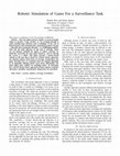A visualization of the iso-concentration contours of the chemical agent is depicted in Fig. 1. B. Problem Formulation We now focus on the inverse problem of determining the parameters of the instantaneous gas release from measurements of the gas concentration. We seek to estimate the location (x0 , y0 ) and time t0 of the explosion, the gas release mass Q, and the eddy diffusivities along the X and Y axes, assumed to be equal, Kx = Ky .1 The wind velocity u is provided by an anemometer and is treated as a known constant. We formulate a least-squares estimation problem for determining the parameter vector θ = [Q Kx x0 y0 t0 ]T , using measurements Zk of the concentration Ck = C(xk , yk , 0, tk ; θ) of the chemical agent corrupted by zeromean white Gaussian noise n(tk ): Zk = Ck + n(tk ) (4)   where σn2 = E n(tk )2 is the variance of this noise. From Eq. (2), the following expression for the natural logarithm of the concentration of the gas is derived:   Q 3 hk (θ) = ln Ck = ln − ln (∆t) 1 3 2 2 2 2 4π (Kx Kz )   1 ∆x2 ∆y 2 + − 4Kx 4Kx ∆t u2 ∆t 2u∆x − + (5) 4Kx 4Kx Note that this formula contains no exponential terms, which greatly simplifies the following derivations. Eq. (5) relates the logarithm of the concentration with the parameter vector θ, defined above. The natural logarithm of each measurement of the concentration, Z̄k , is given by: Z̄k = ln Ck + n(tk ) ≃ ln Ck + n̄(tk ) (6) where n̄(tk ) is a noise process corrupting the logarithm of the concentration. At this point, a comment regarding the distribution of the samples of the noise process n̄(tk ) is necessary. The basic assumption is that the measurement noise is a white, zero-mean, Gaussian process. By plotting a histogram of the samples of this noise process, empirically determined through Monte Carlo simulation as shown in Fig. 2, we observe that the spread of n̄(tk ) can be well approximated by a Gaussian probability density function (pdf). Linearization of Eq. (6) yields n̄(tk ) ≃ 1 n(tk ) Ck (7) Thus the variance σn̄2 (scalar) of n̄ is given by: σn̄2 = E[n̄2 (tk )] = σ2 1 1 E[n2 (tk )] = n2 = 2 2 Ck Ck α (8) where α2 is the constant signal to noise ratio (SNR). 1K z can be found by using models such as those described in [18]. 150 1000 900 100 800 50 700 yc 600 0 500 400 −50 300 −100 200 −150 −150 100 −100 −50 0 xc 50 100 150 0 −1.5 −1 −0.5 0 0.5 1 1.5 2 −5 x 10 Fig. 1. tours. Iso-concentration con- Fig. 2. Log noise histogram. The cost function we seek to minimize is f (θ) = Z̄ − h (θ) T R−1 Z̄ − h (θ) (9)  T where Z̄ = Z̄1 . . . Z̄N is the vector of all (logarithmic) measurements collected by the team of robots, T h(θ) = [ h1 (θ) . . . hN (θ) ] is the vector of the corresponding expected measurements and R = σn̄2 IN ×N is the measurement noise matrix. It is clear that f is a nonlinear function of the elements of θ and cannot be solved in closed-form for θ. Therefore, we resort to linearization of this formula by employing the Taylor series expansion of h(θ) ≃ h(θ̂) + H (θ − θ̂), where H = T is the N × 5 Jacobian matrix H(θ̂) = H T1 . . . H TN of h(θ). Since there are five parameters in the estimated vector θ, a minimum of five (non-degenerate) concentration measurements are required, in order for a unique solution to exist. C. Levenberg - Marquardt Optimization for estimating θ In our implementation, the Levenberg-Marquardt method (L-M) has been employed for the iterative minimization of the cost function in Eq. (9). L-M is a combination of the Gauss-Newton and the Steepest Descent methods. It employs function evaluations and gradient information while estimates of the Hessian matrix are computed as the sum of the outer product of the gradients. The behavior of the L-M method is determined by the positive coefficient µp . For small values of µp , L-M approximates the GaussNewton method, whereas for large values of µp it behaves as a Steepest Descent. Given an initial estimate, from the previous time step, 0 θ̂ k = θ̂ k , a recursive relation for the vector of the estimated m+1 parameters θ̂ k+1 = θ̂ k , where m is the last L-M iteration, can be obtained by employing the following iterative process for the minimization of the linearized cost function in Eq. (9): p+1 θ̂ k = p θ̂ k +  k H Ti H i i=1 k × i=1 µp + 2 · Ik×k α
 p H Ti Zi − hi (θ̂ k ) −1 (10) Note that all quantities related to θ̂, on the right hand side of this equation, are computed using the estimated p parameter vector θ̂ k from the p-th iteration. The covariance matrix of the estimated parameter vector θ̂ k is given by −1  k 1 T Pk = 2 (11) Hi Hi α i=1 IV. T RAJECTORY G ENERATION The selection of the locations that the robots should move to in order to collect the chemical agent concentration measurements is based on the minimization of the uncertainty of the estimated parameter vector θ. This is described by the trace of the expected covariance matrix P̂k+1 , computed in Eq. (11) using the expected values of the matrices H i (j xi , j yi ) for any candidate location(s) (j xi , j yi ) considered by the j th robot for collecting the next measurement(s). Through a large number of simulations we have determined that the trace of the expected covariance matrix is locally concave. Therefore, the selection of the sequence of locations where the measurements should be recorded is based on the minimization of a locally concave function. By employing the following theorem, adapted from [19], we conclude that the optimum solution is achieved at an extreme point in its domain. Theorem 1: Let f be a function defined on the bounded, closed concave set Ω. If f has a minimum over Ω, it is achieved at an extreme point of Ω. Fig. 3 shows that the current position of robot j (indicated by a dashed line) is around the global maximum of the cost function. Based on Theorem 1, a robot should move as far as possible from its current location, towards the boundary of the locally concave function, before it collects the next measurement. Therefore, the robots should move in their environment with their respective maximum velocity j Vmax . Having determined the velocity of the robots, we focus on determining the set of directions of motion j φk , k = 1 . . . N, j = 1 . . . M, (where N, M are the total number of measurements and robots, respectively) that minimize the trace of the expected covariance matrix, P̂k+1 . The spatiotemporal distribution of the measurements Z, processed for determining the parameter vector θ, has a significant impact on the accuracy and the convergence properties of this estimation problem. The collection of measurements at each time instant is performed simultaneously by the team of robots. Thus, if we assume that the team is comprised of M robots,   the recorded measurements, at time instant tk , are Zk = 1 Zk 2 Zk . . . M Zk . It is unrealistic to assume that the measurement times and locations can be selected arbitrarily. Thus, a trajectory generation method must be devised that allows for both accurate and timely estimation of the release parameters. Assume that at time tk , the j th robot is located at position (j xk , j yk ). The robot should be able to move at its 300 LOT Random Walk Chemotaxis Anemotaxis 4 x 10 250 3.9 3.8 3.7 200 3.6 3.5 3.4 150 3.3 3.2 3.1 100 200 150 100 50 50 0 x Fig. 3. −50 −100 −150 −200 200 150 100 50 −50 0 −100 −150 −200 0 y Fig. 4. Robot trajectory. xk+1 = j xk + rj cos j φk , j yk+1 = j yk + rj sin j φk Schematically, the motion of the j th robot from one position to another is depicted in Fig. 4. The same procedure is also followed by the rest of the team. A. Globally Optimal Trajectory (GOT) Several techniques can be applied to generate the optimal trajectories of the robots. Exhaustive search is probably the simplest method and is based on the calculation of all candidate sets of trajectories and choosing the “best” among them. The optimization criterion that is used for the determining the optimal trajectories is the minimization of the trace of the expected covariance matrix. This involves discretizing the reachable set, for each time step and for each robot, into δφd = 2π/d intervals. Thus, if there are N steps along the path, then O(dN ) candidate trajectories must be generated for each robot. If the team is comprised of M robots then the complexity of the problem increases to O(dN M ). It is clear that for large values of M and N this approach is computationally intractable. B. Locally Optimal Trajectory (LOT) A new technique is now described that makes only onestep ahead prediction for the next positions where the robots should move, in order to register the next group of measurements. This approach, referred to hereafter as Locally Optimal Trajectory (LOT), has both reasonable computational cost and convergence time. The iterative one-step optimization process that describes the new motion strategy for collecting the gas concentration measurements, is based on the following recursive criterion: j  −1
j j uk = arg min trace Ak + HT j(k+1) ( φk )H j(k+1) ( φk ) jφ 5 Fig. 5. Cost function representation (3D). maximum velocity j Vmax for some sampling time interval ∆T . This provides a set of reachable points that form a circle of radius rj = j Vmax · ∆T . Thus, the next location for sampling becomes a function of its heading j φk and is provided by the following equations: j 0 (12) k In this relation, the second term H Tj(k+1) (j φk )H j(k+1) (j φk ) is a function of the direction j φk that the j th robot should follow in 10 15 20 25 30 Trace of the covariance matrix. j . Here, Ak = order to collect knext measurement j−1Zk+1 M its T νk I5×5 + i=1 l=1 H il H il + i=1 H Ti(k+1) H i(k+1) , where νk is a small positive number, constant at each step and is computed based on the previous location, j xi , j yi and time instant ti where the j th robot recorded measurements, j Zi , i = 1 · · · k. The term νk I5×5 is used in order to guarantee invertibility ofAk .Furthermore, k M T the second term of Ak , i.e., l=1 H il H il i=1 corresponds to the information due to the previous collected measurements by the robots, while the third j−1 T term i=1 H i(k+1) H i(k+1) represents the expected information that will be contributed by the j − 1 future measurements scheduled to be collected by the j − 1 robots that have already determined the optimal locations for them to go to. The solution to this optimization problem provides the next best sensing position j xk+1 , j yk+1 of the j th robot for minimizing the uncertainty of the estimate θ k+1 . The same procedure is followed by all teammates in order to select their new positions. Once the robots make a decision about their new positions, they move there, record measurements and the procedure starts from the beginning. The same process is repeated until a sufficient number of measurements have been captured in order to reduce the uncertainty of the estimated parameter vector θ below a specific threshold. This method has linear computational cost in terms of the number of measurements and can be implemented on a multi robot system with limited processing capabilities. In [20], we have proven that the cost function in Eq. (12) is equivalent to:   T Hk+1 A−2 k Hk+1 j uk = arg max (13) T φk 1 + Hk+1 A−1 k Hk+1 This form of the cost function can be approximated by: g2 ω 2 + g1 ω + g0 (14) ω (s2 + 2)ω 2 + s1 ω + (s0 + 1)
 k and γk is the bearing angle where ω = tan γk −φ 2 towards the estimated peak of the gas concentration. The scalars gi and si , i = 0, 1, 2, are functions of the problem parameters and are given in [20]. j ∗ uk ≃ arg max 140 12000 60 100 120 90 10000 50 100 4000 50 40 80 0 0 x 6000 60 Time, t (s) 70 Location, x (m) 2 Eddy Diffusivity, K (m /s) Gas Release, Q(Kg) 80 8000 60 30 20 40 40 30 2000 10 20 20 0 1 2 3 4 5 6 7 8 9 10 10 1 2 3 4 Number of Measurements 5 6 7 8 9 0 10 1 2 3 (b) Eddy Diffusivity, Kx . Fig. 6. 60 7 8 1 2 3 4 5 6 7 8 9 10 (d) Time of explosion, t0 . 100 80 Robot 1 Robot 2 Robot 3 Robot 4 Robot 5 Source of Explosion u 60 40 50 0 yc 20 yc 20 yc 0 10 Number of Measurements Robot 1 Robot 2 Robot 3 Robot 4 Robot 5 Source of Explosion u 100 40 0 −20 0 −20 −40 −40 −50 −60 −60 −80 −100 −50 9 Convergence of four, out of five, estimated parameters using LOT. Robot 1 Robot 2 Robot 3 Robot 4 Robot 5 Source of Explosion u 6 (c) Release location, x0 . 100 80 5 Number of Measurements Number of Measurements (a) Mass of released gas, Q. 4 −80 −100 0 50 100 150 −100 −50 0 50 100 −100 −50 0 xc xc (b) u = −0.5m/sec. (a) u = 0.5m/sec. Fig. 7. 50 100 150 xc (c) u = 1.1m/sec Trajectories of the Multi-Robot System for three different values of wind velocity. V. S IMULATION R ESULTS In many real-world scenarios sufficient prior knowledge about some of the parameters of the advection-diffusion equation is unavailable or potentially inaccurate. However, it is likely to have good initial information for some of the estimated parameters. Specifically, for the location of the source x0 , y0 and the time of explosion t0 , satisfactory initial information can be available based on witness reports of the event. In addition, the eddy diffusivity Kx = Ky depends on the atmospheric conditions and the type of the chemical agent. Therefore, an initial approximation about its value can be obtained using precomputed tables. On the other hand, it is almost impossible to have reliable initial information about the value of the mass of the released gas Q. To reflect this, the initial approximation of this parameter has been intentionally selected far from its actual value. We now present a test case of five mobile robots, which move on an flat, obstacle-free terrain without climate variations, having maximum velocity Vmax = 1 m/sec. The initial locations, the starting and sampling time and the known (constant) parameters are shown in Table I, whereas the initial information about the values of the estimated parameters are presented in Table II. Furthermore, the trajectories of the robots for collecting the measurements are presented in Fig. 7. Observing Fig. 6, the elements of the estimated parameter vector θ̂ k converge to their real values even though the initial information θ̂ 0 is inaccurate. Convergence is achieved when the team of robots processes the 5th group of recorded measurements of the gas concentration. Regarding the trajectories of the robots, the LOT approach dictates that robots move along the direction of the wind following the highest point of the gas concentration. This scenario has been addressed using three of the most popular approaches to the odor localization, namely, Chemotaxis, Anemotaxis and Random walk. In Fig. 5, the trace of the covariance matrix for each method, is presented after the second group of measurements was recorded. Observing this figure, the trace of the covariance matrix for the LOT approach converges faster and to a lower value than any of the three aforementioned methods. The same scenario has been implemented for different values of wind velocity. In one case, the wind velocity is u = −0.5 m/sec, whereas in the other case the wind moves faster than robots, i.e., u = 1.1 m/sec. The results for these two cases are shown in Fig. 7. In the first case, three robots move along the direction of the wind, whereas the rest of the team moves in the upwind direction. Considering this, it can be mentioned that some of the robots behave differently from their teammates, even though they operate in the same environmental conditions. Thus, predefining the trajectories of the robots using as the exclusive criteria the characteristics of the wind (i.e., direction, velocity) may not be reliable. In the second case, where the wind velocity is higher than that of the robots, all of them move in the upwind direction for collecting the gas concentration measurements. VI. C ONCLUSIONS This paper presents a new approach for estimating in real-time the parameters associated with an instantaneous gas release in a time crucial situation. Using the advectiondiffusion equation model for the propagation of the gas release, this new approach is a combination of a nonlinear least-squares estimation and a Locally Optimal Trajectory (LOT) generation technique. A team of mobile robots, equipped with sensitive gas sensors and anemometric vanes is used for collecting the chemical agent concentration measurements. Each of the robots communicates and exchanges information about the gas concentration measurements with its teammates. The estimated parameter vector θ̂ converges to its real value even though the initial information θ̂ 0 is inaccurate. VII. ACKNOWLEDGEMENTS This work was supported by the University of Minnesota (DTC), and the National Science Foundation (ITR0324864, MRI-0420836). TABLE I C ONSTANT PARAMETERS . Parameter Mean Wind Velocity Sampling time Initial Position of the robot 1 Initial Position of the robot 2 Initial Position of the robot 3 Initial Position of the robot 4 Initial Position of the robot 5 Initial time Eddy Diffusivity in Z axis Signal to Noise Ratio (SNR) u ∆T x1 (t), y1 (t) x2 (t), y2 (t) x3 (t), y3 (t) x4 (t), y4 (t) x5 (t), y5 (t) t Kz α2 Units m/sec sec m m m m m sec m2 /sec Values 0.5 4 (20,20) (25,25) (10,10) (10,-10) (20,-20) 100 0.2113 103 TABLE II R EAL , I NITIAL , AND E STIMATED VALUES OF THE PARAMETERS . Parameter Gas Release Mass Eddy Diffusivity Location of Explosion Location of Explosion Time of Exposion Q Kx x0 y0 t0 Units Kg m2 /sec m m sec θ 1000 12 2 5 2 θ̂0 600 20 60 40 60 θ̂k 1001.50 12.006 1.9649 5.0707 1.9594 R EFERENCES [1] A. Kalelkar, “Investigation of large-magnitude incidents: Bhopal as a case study,” in Institute of Chemical Engineers, Conference on Preventing Major Chemical Accidents, Cambridge, MA, May 1998. [2] D. Zarzhitsky, D. F. Spears, D. R. Thayer, and W. M. Spears, “Agent- Based Chemical Plume Tracing using Fluid Dynamics,” in Proceedings of Formal Approaches to Agent-Based Systems (FAABS III), 2004. [3] D. Zarzhitsky, D. F. Spears, W. M. Spears, and D. R. Thayer, “A Fluid Dynamics Approach to Multi-Robot Chemical Plume Tracing,” in Proceedings of the Third International Joint Conference on Autonomous Agents and Multi Agent Systems, New York, NY, July 2004. [4] A. Lilienthal, D. Reinmann, and A. Zell, “Gas Source Tracing with a Mobile Robot Using an Adapted Moth Strategy,” in Proceedings of Autonomous Mobile Systems, Stuttgart, Germany, Dec. 2003, pp. 150–160. [5] A. Dhariwal, G. S. Sukhatme, and A. A. G. Requicha, “Bacterium - inspired Robots for Environmental Monitoring,” in Proceedings of the IEEE International Conference of Robotics and Automation, New Orleans, LA, May 2004, pp. 1436–1443. [6] H. Ishida, K. Suetsugu, T. Nakamoto, and T. Moriizumi, “Study of an Autonomous Mobile Sensing System for Localization of Odor Source Using Gas Sensors and Anemometric Sensors,” Sensors and Actuators A, vol. 45, pp. 153–157, 1994. [7] H. Ishida, Y. Kagawa, T. Nakamoto, and T. Moriizumi, “Odor-source localization in the clean room by an autonomous mobile sensing system,” Sensors and Actuators B, vol. 33, pp. 115–121, 1996. [8] R. Russell, D. Thiel, R. Deveza, and A. Mackay-Sim, “A Robotic System to Locate Hazardous Chemical Leaks,” in Proceedings of the IEEE International Conference on Robotics and Automation, Nagoya, Japan, May 1995, pp. 556–561. [9] A. Hayes, A. Martinoli, and R. Goodman, “Swarm Robotic Odor Localization,” in Proceedings of the IEEE International Conference on Intelligent Robots and Systems, Maui, HI, Oct. 2001, pp. 1073– 1078. [10] J. A. Farrell, W. Li, S. Pang, and R. Arrieta, “Chemical Plume Tracing Experimental Results with a Remus A.U.V.” in Proceedings of the Ocean Marine Technology and Ocean Science Conference, San Diego, CA, Sep. 2003. [11] G. Evensen, “The Ensemble Kalman Filter: theoretical formulation and practical implementation,” Ocean Dynamics, vol. 53, no. 4, pp. 343–367, November 2003. [12] G. T. Nofsinger and K. W. Smith, “Plume Source Detection using a Process Query System,” in Proceedings of the Defense and Security Symposium Conference. Bellingham, WA: SPIE, Apr. 2004. [13] H. Versteeg and W. Malalasekera, Introduction to computational fluid dynamics. The finite volume method. Longman Scientific and Technical, 1995. [14] R. M. P. Kathirgamanathan, R. McKibbin, “Source term estimation of pollution from an instantaneous point source,” Research Letters in the Information and Mathematical Sciences, vol. 3, no. 1, pp. 59–67, April 2002. [15] ——, “Sourse release-rate estimation of atmospheric pollution from non-steady point source - part [1]: Source at a known location,” Research Letters in the Information and Mathematical Sciences, vol. 5, pp. 71–84, June 2003. [16] ——, “Source release-rate estimation of atmospheric pollution from a non-steady point source - part [2]: Source at an unknown location,” Research Letters in the Information and Mathematical Sciences, vol. 5, pp. 85–118, June 2003. [17] A. Lilienthal and T. Duckett, “Creating Gas Concentration Gridmap with a Mobile Robot,” in Proceedings of the IEEE International Conference on Intelligent Robots and Systems, Las Vegas, NV, Oct. 2003, pp. 118–132. [18] G.Yeh and C.Hug, “Three-Dimensional Air Pollutant modelling in the Lower Atmosphere,” Boundary-Layer Meteorology, vol. 9, pp. 381–390, 1975. [19] D. Luenberger, Linear and Nonlinear Programming, 2nd ed. Addison-Wesley, 1984. [20] V. N. Christopoulos and S. I. Roumeliotis, “Multi Robot Trajectory Generation for Single Source Explosion Parameter Estimation,” Uviversity of Minnesota, Tech. Rep., July 2004, www.cs.umn.edu/∼vchristo/Chemical MULTI.pdf.