Randomness and metastability in CDMA paradigms
Jack Raymond , David Saad
arXiv:0711.4380v3 [cs.IT] 23 Jun 2008
Aston University, Neural Computing Research Group, Birmingham, B4 7ET, UK
Email: raymonjr@aston.ac.uk
Abstract—Code Division Multiple Access (CDMA) in which the
signature code assignment to users contains a random element
has recently become a cornerstone of CDMA research. The
random element in the construction is particularly attractive in
that it provides robustness and flexibility in application, whilst
not making significant sacrifices in terms of multiuser efficiency.
We present results for sparse random codes of two types, with and
without modulation. Simple microscopic consideration on system
samples would suggest differences in the phase space of the two
models, but we demonstrate that the thermodynamic results and
metastable states are equivalent in the minimum bit error rate
detector. We analyse marginal properties of interactions and also
make analogies to constraint satisfiability problems in order to
understand qualitative features of the decoding and metastable
states. This may have consequences for developing algorithmic
methods to escape metastable states, thus improving decoding
performance.
I. I NTRODUCTION
The area of multiuser communications is one of great interest from both theoretical and engineering perspectives [Ver98].
Code Division Multiple Access (CDMA) is a particular
method for allowing multiple users to access channel resources
in an efficient and robust manner, and plays an important role
in the current standards for allocating channel resources in
wireless communications. CDMA utilises channel resources
highly efficiently by allowing many users to transmit on much
of the bandwidth simultaneously, each transmission being
encoded with a user specific signature code. Disentangling the
information in the channel is possible by using the properties
of these codes and much of the focus in CDMA research is
on developing efficient codes and decoding methods.
A typical CDMA paradigm is that bandwidth is broken
into N discrete Time-Frequency blocks (chips) with each
of K users being assigned a user code (~sk ) known by the
base station, the set of all user codes being s (the code).
The user code gives the amplitude and phase by which to
modulate transmission of the scalar symbol on each chip. The
signal (~y) received on N chips by the base station is then
an interfering (additive) combination of the users’ modulated
symbols corrupted during transmission by a fading factor Fkµ
and some signal noise (νµ ). Assuming perfect synchronisation
of the chips the symbols received on each chip are independent
and given by
yµ = νµ +
K
X
bk Fkµ skµ .
(1)
k=1
We focus on a standard channel type (BIAWGN): the Additive
White Gaussian Noise channel (AWGN), employing Binary
Phase Shift Keying (BPSK). The following parameterisations
are assumed: the scalar symbol sent by user k is a bit bk = ±1
with probability Pbk (b) = 12 ; the noise is Gaussian with zero
mean and variance σ02 for all chips; prefect power control
applies so that the fading factor Fkµ = 1; each code element
sµk = ±A, where A is the amplitude of the transmission
by user k on chip µ. Generalisations of the model most
often consider the requirement for perfect synchronisation and
power control. Real CDMA applications also have to deal with
idiosynchracies in hardware and environmental conditions not
easy to treat in a generalised analysis, this has not prevented
its updake in some modern wireless communication standards.
This paper follows previous theoretical analyses (e.g.
[Tan02], [YT06], [MPT06], [RS07]) in studying codes which
are randomly generated for each system from some ensemble.
The canonical random CDMA ensemble is the dense one in
which all chips are transmitted upon [Ver98]. In the sparse
ensemble we consider here (2) only a small number of chips
O(C) are accessed by each user, a less studied system. However there are a number of reasons why the sparse ensemble
first examined in [YT06] may be more practical, based on
its closer similarity to FH/TH-CDMA and the ability to apply
fast message passing algorithms in decoding. In addition, one
can converge towards the properties of the dense ensemble
by increasing the mean user connectivity C only moderately.
It has been shown, for a sparse connectivity model in which
the mean user connectivity is large but much smaller than K,
that the properties become indistinguishable from the dense
channel in cases where BP converges [GW07].
The sparse codes consist of a sparse connectivity matrix and
a modulation part sampled according to
Y Y
L
L
δxµk + φ(xµk )
(2)
Ps (x) ∝
1−
K
K
µ
k
1
(δx,A + δx,−A ) .
(3)
φ(x) =
2
The modulation of non-zero elements in the codes is described
by φ which can be BPSK (as shown) or unmodulated
√ φ(x) =
δx,A , with the amplitude of transmission (A = 1/ L) chosen
for normalisation purposes so that the Power Spectral density
Q, a representative measure of signal to noise ratio, may be
taken as 1/(2σ02 ). The mean chip and user connectivities are
L and C, respectively, such that the load α = L/C = K/N .
Two problems with the basic sparse ensemble (2) at low
connectivity is significant asymmetry in bandwidth access for
users, with a fraction of users being entirely disconnected.
Analogously the utilisation of chips will not be uniform, with
some chips unutilised. These problems can be overcome by
enforcing regularity of the following forms:
"
!#
N
Y
X
Ps (x) ∝
δ
(1 − δxµk ) − C
,
(4)
∝
τk
τK
µ
k
Y
τ1
[..]
Y
µ
k
"
δ
K
X
(1 − δxµk ) − L
k
!#
, (5)
in addition to modulation though φ. It turns out that constraining users to access exactly C chips (4) is very important
in attaining near optimal performance for high Q, whereas
enforcing, in addition, chip regular access (5) produces only
marginally improved performance [RS07] and may be difficult
to implement in practice. In this paper we consider ensembles
with both chip and user regular constraints (5) throughout
since it makes certain aspects of the analysis simpler; we
anticipate results to be qualitatively similar with only the userregular constraint (4).
The theoretical information capacity, and theory of Bayes
optimal decoding requires knowledge of the likelihood of
transmitted bits
!#
Z Y"
X
P̂~ν (~ω )d~ω (6)
δ yµ −
sµk τk + ωµ
Py~|~b (~τ ) ∝
µ
y1
yµ
yΝ
Fig. 1. The inference problem can be represented by a graphical model: a
Tanner (or factor) graph. Each factor (square) represents an interaction and
each bit (circle) denotes a dynamical variable τk which is to be optimised
given the topology and observable values. The observables in this case are
the signal yµ associated to each node, and the code s–(dashed/solid lines
can be used to indicate modulation by ±A in components sµk ). Above is a
representation for a small sparse regular graph (5,4) with L = 4 C = 3.
Cavity fields combine
h2
h1
Cavity biases combine
yµ
u1
τk
yν
u2
τk
τi
yν
τi
k
where P̂~ν is the assumed chip noise distribution to be
marginalised over. If one considers a Gaussian channel noise
model, of variance (σ0 )2 /β (i.e assumption possibly incorrect
by a factor β), then the righthand side is simplified
!2
Y
X
P~b|~y (~τ ) ∝
exp −βQ yµ −
.
(7)
sµk τk
µ
k
Statistical physics provides a concise framework to analyse
this quantity. First we define a Hamiltonian by connection with
the likelihood
!2
X
X
H(~τ ) = Q
νµ +
sµk (bk − τk )
,
(8)
µ
k
where yµ is written in terms of its constituent components (1)
and τk is a candidate value of the sent bit. From this one can
construct the self-averaging free energy.
+
*
X
1
log
exp{−βH(~τ )} .
(9)
f= −
βN
Fig. 2. The fixed points of the self consistent equations are in quantities h and
u which have an interpretation in terms of messages passed on (sub)graphs
of the graphical model (1). If one knows the log likelihood ratio uµk of
bit bk given only one of its neighbours µ, then assuming these likelihoods
to be independent (as is valid on a tree), one can construct the conditional
likelihood of bk given all its neighbours excluding ν (or log likelihood ratio
hkν ). One can then use hkν to construct log likelihoods (uνi ) for subsequent
variables in the tree. By such a process, the distribution of {h} and {u} may
converge at sufficient depth in the tree to values independent of the inputs –
such a solution is a viable solution to a population dynamics algorithm. The
convergence properties and stability of solutions is closely related to standard
decoding algorithms: the sum product algorithm or belief propagation.
mutual information between the sent bits and the received
signal I(~b, ~y ) and is affine to the free energy. By taking the
limit K → ∞ we are able to attain an exact description
for these fixed points, thereby providing a good indication
of performance. We assume throughout this proceedings that
β = 1, analysis of the free energy thereby corresponds to the
performance of a detector which minimises the bit error rate.
~
τ
The average hi denotes throughout the paper an average over
~y and codes s sampled according to the appropriate ensemble.
The motivation for studying the self-averaged free energy that
this is a generating function for many interesting statistics
attainable by decoders, averaged over samples of the system.
It can be observed that for CDMA the performance measures,
such as bit error rate and spectral efficiency, are self-averaging
– rapidly converging to some fixed values as the number
of users increase. The bit error rate is mean overlap of the
1 ~
h(b.~τ )i, the spectral efficiency is the
sent and decoded bits K
A. Overview of results for BPSK
For sparse ensembles with BPSK the equilibrium and
dynamical properties are similar to the dense case [Tan02],
becoming more so as L increases [GW07]. If one calculates
the free energy of the sparse ensemble by the cavity or replica
method [MPV87] one attains under assumptions of a single
pure state a site factorised expression for the free energy,
determined by the solution to a set of self consistent field
and bias distributions (saddlepoint equations) [RS07]. These
log 10(Probability of bit error)
−1
Spectral Efficiency [bits]
2
−2
2:3
3:3
4:3
5:3
6:3 (Bad)
6:3 (Good)
−3
−4
−5
1.5
1
0.5
−5
0
5
10
Power Spectral Density,Q [dB]
Fig. 3. The figures show the spectral efficiency (affine to the free energy) and
bit error rate for a number of cases of α as indicated by K:N . The solid curves
represent locally stable solutions of the population dynamics procedure for a
sparse ensemble, dashed curves show the exact results for the Q-equivalent
densely spread CDMA system – the curves are qualitatively similar in both
quantities, except in the existence of one additional (unstable) solution in the
dense case (middle curve). The similarity extends to the metastable ranges,
we consider the sparse ensemble results in detail. The sparse ensemble is
fully regular with C = 3 and L = 2, .., 6 in agreement with the ratio α.
For small loads α a unique solution is found in both cases, which is the
valid thermodynamic (information theoretic) solution. For the sparse case at
sufficiently large α (case 6:3) the solution becomes multivalued. Lower figure:
The thermodynamic solution is the curve of lowest spectral efficiency, the
other being metastable; there is a second order transition between the two
solution with increasing Q. The inset shows in detail the region in which
the dense and sparse codes undergo thermodynamic second order transitions
with α = 2. Upper figure: This demonstrates the bit error rate for comparable
parameterisations. This figure indicates a large performance gap between the
two locally stable solutions in the metastable regime: a bad and good solution
exist in terms of decoding. The vertical dashed line indicates the smallest Q
at which metastability occurs in the sparse code for the 6:3 case: beyond
this point in the metastable regime the bad solution performance is typically
attained by belief propagation even if this is only a metastable solution.
results are presented for later comparison (12)
!
Z C−1
C−1
i
X
Yh
uc
duc Ŵ (uc ) δ h −
W (h) ∝
c=1
c=1
Ŵ (u) ∝
Z L−1
Y
[W (hl )dhl ]
l=1
× δ u−
L
Y
B. A sparse model without modulation
[φ(xl )dxl ] Pν (ω)dω
l=1
X
!
τL log(Z(τL ))
τL
(10)
!2
L
X
X
X
Z(τL ) =
exp −Q ω +
xl (1 − τl ) +
hl τl
~
τ
l=1
fields h. These variables may be interpreted within a graphical
framework of the inference problem (Fig. 1), as log-likelihood
(of correct decoding) ratios in two types of sub-graphs (Fig. 2).
From these distributions one can calculate the free energy,
bit error rate and other properties. The equations may be
solved numerically by population dynamics [RS07], which is
implemented as a late propagation (decoding) algorithm on
a tree. This processes allows a numerical determination of
the free energy and tests of ergodicity breaking. We find a
unique thermodynamic solution at all Q, but also a significant
metastable solution for a range of parameters (Fig. 3).
We may distinguish the metastable states in this range
of parameters as bad and good (higher or lower bit error
rate). The population dynamics algorithm tends to find the
bad solution from most initial conditions, only those initial
conditions which are of very low bit error rate (a set of
cavity biases strongly correlated with ~b) appear to converge
towards the good solution. It appears the bad solution is easy
to reach by implementation of population dynamics regardless
of whether it is the thermodynamically dominant state. This is
interesting since population dynamics appears to mirror the
behaviour of many decoding algorithms on even relatively
small systems, which struggle to achieve good bit error rates
in this region. In the real decoding problem one does not begin
the decoding already with a good estimate of ~b, and so one may
be stuck with a suboptimal estimate even where a much better
estimate may be found (in principle) for almost all decodings.
In both the dense and sparse cases there is a unique
thermodynamically stable state. One can hope to achieve the
information capacity of the thermodynamic state by clever
algorihms based on some global insight. The problem is that
local search based optimisation appears insufficient. In the case
of no metastability, local search methods attain the optimal solution [GW07], [RS07] with various principled modifications
suggested [Kab03]. In the case of metastability one might
apply a principle of guesswork combined with BP to allow
efficient searching of the space. Such a method [MMU05] has
been demonstrated for certain types of channel, unfortunately
not so far the BIAWGN we consider. In the following sections
we consider how the similarity between the phenomena in
dense and sparse systems, combined with a consideration of
marginal interaction distributions, might characterise the bad
metastable solution and how such insight might be used to
supplement local search methods.
l
where Pν is the true chip noise probability distribution. The
distributions are over a set of cavity biases u and cavity
As a way to further understand the microscopic basis of
metastability we propose the following model to investigate the
sparse ensemble for the case of no modulation, φ(x) = δx,A .
Unlike the dense model, the disorder in the connectivity
structure is sufficient to recover information even without
modulation. Given that the graphical structure is identical to
the modulated sparse ensemble, decoding may be achieved by
similar methods (belief propagation based local search).
Working with either the cavity or replica methods one can
attain a site factorised set of functional relations analogous to
(10). In the former case we had two distributions containing
information on the probabilty of correct bit reconstruction (on
two types of subgraph). In the unmodulated case we replace
each of these distributions by two, because the probability of
correct bit recovery is dependent on the candidate bit at the
given site, τk = a. Assuming no ergodicity breaking one can
attain the variational part of the free energy density ((9) in the
large N limit) as
XZ
f =
dhduW (a, h)Ŵ (a, u) log(1+tanh(u) tanh(h))
a
+ α
X
a
+
+
ZI =
Z
Pb (a) C duW (a, u) log(cosh u)
Z Y
C
Z
C
X
[duc W (a, uc )] log cosh
c=1
"
L
Y
c=1
X
dxl dφ(xl )
al
l=1
(11)
#
dhl W (al , hl ) dωPν (ω) log ZI
!2
L
X
exp(hl τl )
exp −Q ω + xlal(1−τl )
.
2cosh(hl )
L
XY
~
τ l=1
uc
!!)
l=1
Here Pb is the true prior on transmitted bits, which we will
assume to be uniform. We also assume the sparse ensemble
with chip and user regularity for brevity. The distributions must
be chosen to minimise the free energy, it is a near identical
minimisation which gives rise to (10). The pairs of field and
bias distributions Ŵ ,W , in this case obey the saddlepoint
equations
!
Z C−1
C−1
i
X
Yh
uc
duc Ŵ (a, uc ) δ h −
W (a, h) ∝
c=1
c=1
#
"
Z L−1
Y
X
φ(xl )dxl
Ŵ (aL , u) ∝
W (al , hl )dhl Pν (ω)dω
al
l=1
× δ
u−
X
τL
!
τL log(Z(τL ))
(12)
Where Z is the same quantity as (10) upto the substitution
of xl by al . In this new case we have a modified set of
equations on distributions, as the dependence on the root site
cannot be factorised. Since we are considering maximal rate
both in the prior for sent message and inference model we
can argue by symmetry that W (b, h) equals W (−b, h). This
represents the intuitive statement that the probability of correct
reconstruction is independent of whether the sent bit is ±1,
however this is an ansatz rather than a result of the calculation. The assumption can be tested by allowing convergence
restricted to the symmetric combination and testing small
perturbations in the antisymmetric part. A stronger test of the
ansatz is to allow the population dynamics to run with fully
independent distributions. To within numerical accuracy the
restricted solutions and those found in this larger space appear
to be consistent and the modulated and unmodulated sparse
ensembles become equivalent. At maximal rate the solution
for the unmodulated ensemble is information theoretically
equivalent to the unmodulated ensemble.
II. NATURE
OF THE METASTABLE SOLUTIONS
The exact results and numerical solutions (as indicated by
example in Fig. 3) indicate several common features of the
metastable state for both the sparse and dense systems. We
investigate these points and present some simplified analysis
of the energy landscape in this section. The results of the
previous section provide insight into the probable nature of
the state, and the fact that the sparse and dense systems
are so similar qualitatively means that topology must play a
relatively small role. The dynamical properties of the decoding
algorithms reported for both cases appear to be an important
common feature, while the sizes of solutions (as indicated by
entropy) and bit error rates reduce the space of solutions to
be considered.
A. Predictions for decoding failure in the marginal fields and
couplings
One can gain further insight by examining the interaction
structure as a source of information, making analogies between other well studied disordered systems [MPV87]. The
Hamiltonian may be re-written (upto constants) as
X
X
H(~τ ) = −
(13)
Jkk′ τk τk′ +
hk τk
k6=k′
k
which is a standard formulation in physics, where the set of
couplings Jij and fields hi describe the problem
X
Jk,k′ = −Q
(14)
sµk sµk′
µ
hk = 2Q
X
yµ sµk = 2Q
µ
"
X
µ
s2µk
#
bk
(
)
X
X
X
+ 2Q
sµk′ bk′ } +
sµk
νµ sµk }
′
µ
k (6=k)
µ
Since the coupling term has no dependence on the sent bits ~b
the states induced by the couplings alone must be uncorrelated
with the true solution. By contrast, the field term encodes a
bias towards the sent vector combined with a pair of fields
with no alignment along the correct solution (in expectation),
but with some dependence thereof.
The couplings and fields are strongly correlated through
the code s. In the case of a dense code where L → K both
marginal distributions over couplings and fields may be taken
as Gaussian distributed through application of the central limit
theorem with N = K/α large; the dense case gives
Q2
,
(15)
P (Jk,k′ ) = N 0,
αN
2Qbk (2Q)2
2Q
P (hk ) = N
.
(16)
,
+
α
α
α
where N signifies the normal distribution. The first term of
the field variance is negligable for the large system.
For the sparse code with BPSK one can instead
note that the
couplings are non-zero with probability L2 / K
L reflecting the
enforced topology (2),(4),(5), and in the non-zero cases take
values ±Q/L with equal probability. In the field part one has
a net positive field combined with two terms, the first term
containing no noisy part gives a variance dependent on the
site values and number of nearest neighbours (users connected
through chips to user k), whereas the second is the sum of
Gaussian random variables associated to each neighbouring
chip. We approximate the distribution by a mean and variance
to abbreviate this information, ignoring for convenience higher
order moments as
2Q
(2Q)bk (L − 1)(2Q)2
,
+
.
(17)
P (hk ) = N
α
αL
α
The L−1 prefactor is the average excess degree of the factor
node in the chip regular ensemble (5), for the random graph
ensemble (2) the value is L (also with user regularity (4)).
Using a non-regular code appears to impact upon the variance
of the field but not the mean.
When one does not include the BPSK, the first two moments
of the sparse distribution of local fields (17) are unchanged
but the couplings are entirely anti-ferromagnetic Q/L, again
conforming to the underlying topology. At least for β = 1
we have determined that the information theoretical quantities,
and the population dynamics algorithm are equivalent for the
two sparse ensembles considered. Therefore we expect only
features common to the two models to be responsible for
the metastability and other non-trivial properties in the large
system limit.
We can now consider common features in the distributions.
In so far as a marginalised distribution might provide insight, it
appears fairly clear that there is a competition between a mean
dominated field producing good reconstruction and a variance
dominated field leading to only marginal bias in favour of
correct reconstruction. The field presumably projects into one
of a number of local minima. When Q is small the variance
dominates and there is a weak net alignment with ~b. As one
increases Q the mean grows more quickly than the spread, so
that in the large Q limit the state is very orderly. By contrast
as one increases α the mean is suppressed by comparison with
the spread in the field (and in the couplings), so that one might
expect the state to be variance dominated.
The marginal coupling distributions appear very different
in the modulated models (sparse and dense) by comparison
the unmodulated model. In the modulated model one has
a random coupling, which one might expect would induce
behaviour comparable to a random spin glass or an inverse of
the Hopfield model [MPV87], with a highly non-trivial distribution of local solutions (when ignoring the field). However,
by investigation of the unmodulated model we see the space
determined entirely by the couplings is in no way related to
the modulation pattern, and hence the source of metastability
cannot relate to this for our detector in the sparse case, the
Hopfield analogy is certainly not useful. The second model is
a random field Ising anti-ferromagnet, the former is a random
field spin-glass, if the structure were a random graph with
uncorrelated spin-spin edges (a Viana Bray model) we might
expect behaviour to be quite comparable and described by a
complicated energy landscape with many local minima – in the
absence of topological features the presence of metastability
should not be a surprise, what is a surprise is that it appears for
only a small range of parameters and has a bi-modal structure.
B. Sources of metastability by analogy with CSPs
What is important not to overlook in the above marginal
link and field description is a consideration of the strong local
correlations in graph topology, the interactions are formed
in local cliques (fully connected sets of L variables) and
not independently. Although the fields are generated from an
unusual ensemble they cannot be responsible for metastability,
since in themselves they generate no long range correlations.
We can first consider the role of couplings in the absence of
a field. If one considers the details of the interaction structure
one can observe that the ground state is closely related to
random constraint satisfiability problems (CSP) [MPV87] such
as the ’not all equal satisfiability’ (NAE-SAT) model. Suppose
chip connectivity of L = 3 for all chips (hyperedges) in the
system with an unmodulated sparse code, then the energy for
the clique of dynamic variables (spins) attached to chip µ is
P
bk bk′ in the coupling part (13). This gives chip energy of
either 3, with all (modulated) spins equal, or −1 for any other
assignments. The set of spin-assignment which simultaneously
produces the fewest all equal cases (closest to the not all equal
case satisfied case) are the ground state(s) of the system. The
random NAESAT model is known to have a ground state set
which is algorithmically non-trivial to find with variation of
α [ACIM01]. The fragmentation of the space (clustering) is
understood to cause these features in many CSPs and statistical
physics can produce exact descriptions of the correlations and
other features of the thermodynamic solution. Figure 3 might
be expected to reveal some corresponding phase transition
in the underlying CSP with variation of α. Thermodynamic
features of the ground state correspond to properties of a
maximum likelihood detector, which is closely related to the
minimum bit error rate detector we analyse.
Finally we must introduce the fields, afterall this is where
the information about the transmitted bits exist. The field
effectively define a vector in the energy landscape, and the
energy must be minimised with respect to this direction (the
energy landscape is effectively rotated). Using this analogy
we can understand that the metastability arises out of the
clustering of the underlying CSP reorientated by the field. One
begins the search for the lowest energy in the vicinity of the
matched-filter (field determined) solution, the local solution
close to the encoded solution may be thermodynamically
optimal but if the field projection is not into the cluster then
local search methods are certain to fail. In solution spaces cf
disjoint clusters one must work in a low noise regime, the field
then almost certainly projects very close to the best state and
local search is successful. This observation is consistent with
the disappearance of suboptimal solutions at sufficiently high
signal to noise ratios for all ensembles.
III. C ONCLUSION
A comparison of the marginal coupling distributions in
the two sparse cases indicates a substantial difference unlike
a comparison between sparse and dense modulated code
ensembles. The quadratic Hamiltonian form seems to predict
the appropriate regimes where decoding performance is weak
by consideration of only the fields. The contrast between the
two sparse ensembles suggests variance in the field is the most
important factor in preventing successful decoding. In one case
the couplings are similar to those of a sparse spin glass, in
the other the couplings are uniform, but anti-ferromagnetic.
When local topology is considered we see a connection to
constraint satisfiability problems, which is a more convincing
explanation of the origins of metastability. To avoid metastable
states in decoding we might hope to make use of the fact
that we know the suboptimal states induced by the couplings
are related to random CSPs, the ground states of which are
for some parameterisations exactly solvable even on loopy
graphs (with high probability), or have a well understood
(asymptotic) state space structure. With a fragmented state
space local search algorithms such as belief propagation may
not converge, and other heuristic methods may be appropriate
using a detailed knowledge of the CSP for example. It would
also be interesting to further investigate what similarities exist
between the modulated and unmodulated sparse codes in a
wider range of detectors. The equivalence of modulated and
unmodulated sparse codes in the minimum bit error rate
detector should not apply to other detection methods or finite
size systems, and hence in terms of practical performance of
codes we may expect one ensemble to outperform the other.
ACKNOWLEDGMENT
Support from EVERGROW, IP No. 1935 in FP6 of the EU
and EPSRC grant EP/E049516/1 are gratefully acknowledged.
R EFERENCES
[ACIM01] Achlioptas D, Chtcherba A D, Istrate G and Moore C, The phase
transition in 1-in-k SAT and NAE 3-SAT, 2001 SODA, 721-722,
[GW07] D. Guo and C. Wang. Multiuser detection of sparsely spread cdma.
(unpublished), 2007.
[Kab03] Y. Kabashima. A cdma multiuser detection algorithm on the basis
of belief propagation. Jour. Phys. A, 36(43):11111–11121, 2003.
[MMU05] C. Measson, A. Montanari and R. Urbanke. Maxwell Construction: The Hidden Bridge between Iterative and Maximum a Posteriori
Decoding. Preprint arXiv:cs/0506083, 2005.
[MPT06] A. Montanari, B. Prabhakar, and D. Tse. Belief propagation
based multiuser detection. In Proceedings of the Allerton Conference
on Communication, Control and Computing, Monticello, USA, 2006.
[MPV87] M. Mezard, G. Parisi, and M.A Virasoro. Spin Glass Theory and
Beyond. World Scientific, 1987.
[RS07] J. Raymond and D. Saad. Sparsely spread CDMA - a statistical
mechanics-based analysis Jour. Phys. A, 40(41),12315-12334,2007.
[Tan02] T. Tanaka. A statistical-mechanics approach to large-system analysis
of cdma multiuser detectors. Information Theory, IEEE Transactions on,
48(11):2888–2910, Nov 2002.
[Ver98] S. Verdu. Multiuser Detection. Cambridge University Press, New
York, NY, USA, 1998.
[YT06] M. Yoshida and T. Tanaka. Analysis of sparsely-spread cdma via
statistical mechanics. In Proceedings - IEEE International Symposium
on Information Theory, 2006., pages 2378–2382, 2006.
Keep reading this paper — and 50 million others — with a free Academia account
Used by leading Academics

Jorge Eterovic
Universidad Nacional de la Matanza

Mehmet Hilal Özcanhan
Dokuz Eylül University

Paul Tobin
Dublin Institute of Technology

Monish Chatterjee
University of Dayton