arXiv:0904.2265v1 [nlin.SI] 15 Apr 2009
Factorized finite-size Ising model spin matrix
elements from Separation of Variables
G von Gehlen† , N Iorgov‡ , S Pakuliak♯♭ and V Shadura‡
†
Physikalisches Institut der Universität Bonn, Nussallee 12, D-53115 Bonn, Germany
Bogolyubov Institute for Theoretical Physics, Kiev 03680, Ukraine
♯
Bogoliubov Laboratory of Theoretical Physics, Joint Institute for Nuclear Research,
Dubna 141980, Moscow region, Russia
♭
Institute of Theoretical and Experimental Physics, Moscow 117259, Russia
‡
E-mail: gehlen@th.physik.uni-bonn.de, iorgov@bitp.kiev.ua,
pakuliak@theor.jinr.ru, shadura@bitp.kiev.ua
Abstract. Using the Sklyanin-Kharchev-Lebedev method of Separation of Variables
adapted to the cyclic Baxter–Bazhanov–Stroganov or τ (2) -model, we derive factorized
formulae for general finite-size Ising model spin matrix elements, proving a recent
conjecture by Bugrij and Lisovyy.
15 April 2009
Submitted to: J. Phys. A: Math. Gen.
PACS numbers: 75.10Hk, 75.10Jm, 05.50+q, 02.30Ik
1. Introduction
Much work has been done on the 2-dimensional Ising model (IM) during the past over
60 years. Many analytic results for the partition function and correlations have been
obtained. These have greatly contributed to establish our present understanding of
continuous phase transitions in systems with short range interactions [1, 2, 3, 4, 5, 6].
Recent overviews with many references are given e.g. in [7, 8, 9]. Many rather different
mathematical approaches have been used, so that already 30 years ago Baxter and
Enting published the “399th” solution for the free energy [10], see also [11]. Spin-spin
correlation functions can be written as Pfaffians of Toeplitz determinants. Most work
has focussed on the thermodynamic limit and scaling properties since these give contact
to field theoretical results and to beautiful Painlevé properties [5, 6, 12].
Only during the last decade more attention has been drawn to correlations and spin
matrix elements (form factors [13]) in finite-size Ising systems [14, 15, 16]. Nanophysics
experimental arrangements often deal with systems where the finite size matters.
Recent theoretical work on the finite-size IM started from Pfaffians and related Clifford
approaches. In [17] it has been pointed out that one may write completely factorized
closed expressions for spin matrix elements of finite-size Ising systems. One goal of the
present paper is to prove the beautiful compact formula conjectured in Eq.(12) of [17],
�Ising model spin matrix elements from Separation of Variables
2
see (129). For achieving this, we introduce a method which has not yet been applied to
the Ising model: Separation of Variables (SoV) for cyclic quantum spin systems. Our
approach is the adaption to cyclic models of the method introduced by Sklyanin [19, 20]
and further developed by Kharchev and Lebedev [21, 22]. We also make extensive use
of the analysis of quantum cyclic systems given in [23].
Little is known about state vectors of the 2-dimensional finite-size IM. Only partial
information about these state vectors can be obtained from the work of [3]. Recently
Lisovyy [24] found explicit expressions using the Grassmann algebra method. Here we
shall present our SoV approach [25, 26, 27] which gives explicit formulas for finitesize state vectors too. However, these come in a basis quite different from the one
used in [24]. We shall calculate spin matrix elements by directly sandwiching the spin
operator between state vectors. Factorized expressions result if we manage to perform
the multiple spin summations over the intermediate states.
The prototype of a general N-state cyclic spin model is the Baxter–Bazhanov–
Stroganov model (BBS) [28, 29, 30], also known as the τ (2) -model. The standard IM is
a very special degenerate case of the BBS model. In order to avoid formulating many
precautions necessary when dealing with the very special IM, we shall develop our version
of the SoV machinery considering the general BBS model. We chose to do this also
because of the great interest in the BBS model due to the fact that its transfer matrix
commutes with the integrable Chiral Potts model (CPM) [31, 32] transfer matrix [29, 33].
Obtaining state vectors for the CPM is a great actual challenge [34, 35]. Although the
eigenvectors for the transfer matrix of the BBS model with periodic boundary condition
are unknown for N > 2, explicit formulas for the eigenvectors of the BBS model with
open and fixed boundary conditions have been found [36, 37].
This paper is organized as follows: In section 2 we define the BBS model and
its Ising specializations. In section 3 we discuss the Sklyanin SoV method adapted
to the BBS model as a cyclic system. We start with the necessary first step, the
solution of the associated auxiliary problem. In a second step we obtain the eigenvectors
and eigenvalues of the periodic system by Baxter equations. The conditions which
ensure that the Baxter equations have non-trivial solutions are formulated as truncated
functional equations. Section 4 gives a description of local spin operators in terms of
global elements of the monodromy matrix. Starting with Section 5 we restrict ourselves
to the case N = 2, for which the BBS model becomes a generalized 5-parameter
plaquette Ising model. In section 6 we further specialize to the homogenous case
and then to the two-parameter Ising case. Periodic boundary condition eigenvectors
are explicitly constructed. Section 7 is devoted to our main result, the proof of the
factorized formula for Ising spin matrix elements between arbitrary finite-size states.
This is shown to agree with the Bugrij-Lisovyy conjecture. In section 8 we give an
analogous formula for the Ising quantum chain in a transverse field. Finally, section 9
presents our Conclusions. Large part of this paper relies on our work in [25, 26, 27].
Sections 4, 2.2 and 6.2 give new material.
�Ising model spin matrix elements from Separation of Variables
3
2. The BBS τ (2) -model
2.1. The inhomogenous BBS-model for general N
We define the BBS-model as a quantum chain model. To each site k of the quantum
chain we associate a cyclic L-operator [29, 30] acting in a two-dimensional auxiliary
space
1 + λκk vk ,
λu−1
(a
−
b
v
)
k
k k
k
, k = 1, 2, . . . , n. (1)
Lk (λ) =
uk (ck − dk vk ), λak ck + vk bk dk /κk
λ is the spectral parameter, n the number of sites. There are five parameters κk ,
ak , bk , ck , dk per site. uk and vk are elements of an ultra local Weyl algebra, obeying
uj uk = uk uj ,
uj vk = ω δj,k vk uj ,
vj vk = vk vj ,
ω = e2πi/N ,
N
uN
k = vk = 1.
At each site k we define a N-dimensional linear space (quantum space) Vk with the basis
|γik , γ ∈ ZN , the dual space Vk∗ with the basis k hγ|, γ ∈ ZN , and the natural pairing
′
∗
k hγ |γik = δγ ′ ,γ . In Vk and Vk the Weyl elements uk and vk act by the formulas:
uk |γik = ω γ |γik , vk |γik = |γ + 1ik ;
k hγ|uk
= k hγ| ω γ ,
k hγ|vk
= k hγ − 1| .
(2)
The monodromy Tn (λ) and transfer matrix tn (λ) for the n sites chain are defined as
!
An (λ) Bn (λ)
Tn (λ) = L1 (λ) · · · Ln (λ) =
, tn (λ) = tr Tn (λ) = An (λ) + Dn (λ). (3)
Cn (λ) Dn (λ)
This quantum chain is integrable since the L-operators (1) are intertwined by the twisted
6-vertex R-matrix at root of unity
λ − ων
0
0
0
0
ω(λ − ν) λ(1 − ω)
0
R(λ, ν) =
(4)
,
0
ν(1 − ω)
λ−ν
0
0
0
0
λ − ων
(1)
(2)
(2)
(1)
R(λ, ν) Lk (λ)Lk (ν) = Lk (ν) Lk (λ) R(λ, ν),
(1)
(5)
(2)
where Lk (λ) = Lk (λ) ⊗ I, Lk (λ) = I ⊗ Lk (λ). Relation (5) leads to [tn (λ), tn (µ)] = 0 .
So tn (λ) is the generating function for the commuting set of non-local and non-hermitian
Hamiltonians H0 , . . . , Hn :
tn (λ) = H0 + H1 λ + · · · + Hn−1 λn−1 + Hn λn .
(6)
From (5) it also follows that the upper-right entry Bn (λ) of Tn (λ) is the generating
function for another commuting set of operators h1 , . . . , hn :
[ Bn (λ), Bn (µ) ] = 0,
Bn (λ) = h1 λ + h2 λ2 + · · · + hn λn .
(7)
Observe that H0 and Hn can be easily written explicitly in terms of the global ZN -charge
rotation operator Vn
n
n
n
Y
Y
Y
bk dk
κk ,
Vn = v1 v2 · · · vn . (8)
ak ck + Vn
,
Hn =
H0 = 1 + Vn
κk
k=1
k=1
k=1
�Ising model spin matrix elements from Separation of Variables
4
Here we shall not explain the great interest in the BBS-model due to a second
intertwining relation in the Weyl-space indices found in [29] and the related fact that for
particular parameters the Baxter Q-operator of the BBS-model is the transfer matrix
of the integrable Chiral Potts model, see [29, 33, 38]. We will also not discuss the
generalizations of the BBS model introduced by Baxter in [39], and not explain how (1)
arises in cyclic representations of the quantum group Uq (sl2 ), see e.g. [23, 40, 41].
The transfer matrix (3) can be written equivalently as a product over face
Boltzmann weights [28, 33]:
Q
′
′
tn (λ) = n+1
k=2 Wτ (γk−1 , γk , γk , γk−1 ) with the face Boltzmann weights
P
′
′
Wτ (γk−1 , γk , γk−1
, γk′ ) = 1mk−1 =0 ω mk−1 (γk −γk−1 )
′
′
′
(γk−1 − γk−1
, mk−1 ) Fk′′ (γk − γk′ , mk−1 )
× (−ωtq )γk −γk −mk−1 Fk−1
(9)
where mk ∈ {0, 1} and Fk′ (∆γ, mk ) = Fk′′ (∆γ, mk ) = 0 if ∆γ 6= {0, 1}, and the nonvanishing values are
!
!
1
λ ak
1
λ ck
′
′′
Fk =
, Fk =
.
(10)
κk −bk /ω
1 −dk /κk
The vanishing of Fk′ (∆γ, mk ) and Fk′′ (∆γ, mk ) for ∆γ 6= {0, 1} means that the vertically
neighboring ZN -spins cannot differ by more than one. The equivalence to the transfer
matrix defined by (1) and (3) is seen writing the matrix elements of (1) as
′
′
hγk′ |Lk (λ)mk−1 ,mk |γk i = ω mk−1 γk −mk γk λγk −γk −mk−1 Fk′′ (γk′ − γk , mk−1 )Fk′ (γk′ − γk , mk ). (11)
Lk
•
•
′
∈ ZN
γk−1
mk−2
•
•
•
γk′
•γ
k−1
•
Fk′
F ′′k
•
γk ∈ ZN
•
•
mk−1
′
Fk−1
γk′
•
mk ∈ Z 2
•
mk−1
•
F ′′k
F ′k
mk
•
•
γk ∈ ZN
Figure 1. Illustration of the two versions: left we see the W of (9) indicated by full
lines, whereas (3) the Lk of (1) arise if we look at the lattice formed by the dashed
lines in the left figure and the dashed rhombus shown at the right. The lattice is built
by ZN -spins on the full lines and Z2 -spins in the centers.
2.2. Homogenous BBS-model for N = 2
The integrability of the BBS-model is valid also if the parameters κk , ak , . . . , dk vary
from site to site and the construction of eigenvalues and eigenvectors can be performed
�Ising model spin matrix elements from Separation of Variables
5
for this general case. However, in order to obtain compact explicit formulas for matrix
elements, we shall often put all parameters equal: κk = κ, . . . , dk = d and call this the
homogenous model. In [42] it has been shown that for N = 2 the general homogenous
BBS-model can be rewritten as a generalized plaquette Ising model with Boltzmann
weights
�
�
P
W (σ1 , σ2 , σ3 , σ4 ) = a0 1 + 1≤i<j≤4 aij σi σj + a4 σ1 σ2 σ3 σ4 ,
(12)
subject to the free-fermion condition a4 = a12 a34 − a13 a24 + a14 a23 .
For N = 2 the Weyl elements can be represented by Pauli matrices. Fixing κ = 1
the L-operator becomes
!
λ σkz (a − b σkx )
1 + λ σkx
Lk (λ) =
σkz (c − d σkx ) λac + σkx b d
degenerating at λ = b/a:
Lk (b/a) =
1 + b/a σkx
σkz (c − dσkx )
!
�
�
1 , b σkz .
The matrix elements of the corresponding transfer-matrix are
n
Y
�
′
δσk ,σk′ (1 + b c σk−1 σk′ ) + δσk ,−σk′ b/a (1 − a d σk−1 σk′ ) ,
h{σ } | tn(b/a) | {σ}i =
k=1
where {σ} = {σ1 , . . . , σn } and {σ ′ } = {σ1′ , . . . , σn′ } are the values of the spin variables
′
of two neighboring rows, σk = (−1)γk , σk′ = (−1)γk ∈ {+1, −1}, and the identifications
′
σn+k = σk , σn+k
= σk′ are used.
•
′
σk−1
•
Kd
•
•
•
Ky
Kx
σk−1
σk′
•
σk
Figure 2. Transfer-matrix for the triangular Ising lattice. Solid lines show the
interaction between spins.
The matrix elements of the transfer-matrix of the Ising model on the triangular
lattice (see Fig. 2) are
′
h{σ }|t△ |{σ}i =
n
Y
k=1
exp(Kx σk−1 σk + Ky σk σk′ + Kd σk−1 σk′ ) .
(13)
�Ising model spin matrix elements from Separation of Variables
6
The k-th factor of this product, taken at σk = σk′ is
exp(Ky ) exp((Kx + Kd ) σk−1 σk′ ) =
= exp(Ky ) cosh(Kx + Kd ) (1 + tanh(Kx + Kd ) σk−1 σk′ ) ,
and at σk = −σk′ is
exp(−Ky ) exp((Kd − Kx ) σk−1 σk′ ) =
= exp(−Ky ) cosh(Kd − Kx ) (1 + tanh(Kd − Kx ) σk−1 σk′ ) .
Now it is easy to compare the transfer-matrices tn (b/a) and t△ :
t△ = exp(nKy ) coshn (Kx + Kd ) tn (b/a) ,
tanh(Kx + Kd ) = b c ,
exp(−2Ky )
cosh(Kd − Kx )
= b/a ,
cosh(Kd + Kx )
tanh(Kx − Kd ) = a d .
Although we considered tn (λ) at the special value of the spectral parameter λ = b/a,
the transfer-matrix eigenstates are independent of this choice of λ. So the eigenstates
of the transfer-matrix of the Ising model on the triangular lattice appear as eigenstates
of the general homogenous BBS-model for N = 2 (the parameter κ and one of the
parameters a, ..., d in the case of homogeneous periodic BBS model can be absorbed
by a rescaling of the other parameters and using a diagonal similarity transformation of
the L-operators). The formulas for them will be given later. Unfortunately, factorized
formulas for the matrix elements of the spin operator in this general case have not been
found. There are only two special cases for which such formulas are available:
• Row-to-row transfer-matrix for the Ising model on the square lattice:
a = c,
b=d:
Kd = 0,
e−2Ky = b/a ,
tanh Kx = a b .
(14)
This case will be the main object of our attention. It is the most general case
where we have the factorized formula for the spin operator matrix elements found
by Bugrij and Lisovyy.
• Diagonal-to-diagonal transfer-matrix for the Ising model on the square lattice:
a = c,
b = −d :
Kx = 0,
e−2Ky = b/a ,
tanh Kd = a b .
(15)
It is known [43] that such transfer-matrices with different parameters Ky = L,
Kd = K (and corresponding a, b) constitute a commuting set of matrices having
common eigenvectors provided
1
a2 − b2
=
(16)
1 − a2 b2
k′
is fixed. Thus in this case the eigenvectors depend on k′ only. Therefore, in order
to find the eigenvectors and the corresponding matrix elements of the spin operator
it is sufficient to fix a = c = 1/(k′ )1/2 and b = d = 0 and so to obtain a special
case of the formulas for the row-to-row transfer-matrix of the Ising model on the
square lattice. Note that we get [27] the same matrix elements in the case of the
sinh 2K sinh 2L =
�Ising model spin matrix elements from Separation of Variables
7
quantum Ising chain in a transverse field with strength k′ because the corresponding
Hamiltonian commutes with the transfer-matrices having the same k′ . Another
remark: with the restriction a = c, b = −d, κ = 1, the transfer-matrices commute
among themselves at independent values of two spectral parameters: λ and the
parameter which uniformizes (16) (a parameter on the elliptic curve with modulus
k′ , see [43]).
3. Separation of Variables for the cyclic BBS-model
3.1. Solving the auxiliary system (7): Eigenvalues and eigenvectors of Bn (λ).
We start giving a summary of the SoV method as applied to the general inhomogenous
ZN -BBS model [25]. The aim is to find the eigenvalues and eigenstates of the n-site
periodic transfer matrix tn (λ) of (3), and the idea [19, 20, 21, 22] is first to construct
a basis of the N n -dimensional eigenspace from eigenstates of Bn (λ), see (7). This can
be done by a recurrent procedure. Then the eigenstates of tn (λ) are written as linear
combinations of the Bn (λ)-eigenstates. The multi-variable coefficients are determined
by Baxter T −Q-equations which by SoV separate into a set of single-variable equations.
From (7) the eigenvalues of Bn (λ) are polynomials in the spectral variable λ.
Factorizing this polynomial, for n ≥ 2 we get
Bn (λ) |Ψλi = λλ0
n−1
Y
k=1
(λ − λk ) |Ψλi;
λ = {λ0 , λ1 , . . . , λn−1 },
(17)
where λ1 , λ2 , . . . , λn−1 are the n − 1 zeros of the eigenvalue polynomial and λ0 is a
normalizing factor. We can label the eigenvectors by λ.
An overview of the space of eigenstates of Bn (λ) is easily obtained using the
intertwining relations (5). It follows from (5) that the operators An (λ) and Dn (λ)
of the monodromy (3), taken at a zero λ = λk , are cyclic ladder operators with respect
to the kth component of λ in |Ψλi. To see this consider e.g. the intertwining relation
(λ − ωµ)An (λ)Bn (µ) = ω(λ − µ)Bn (µ)An (λ) + µ(1 − ω)An (µ)Bn (λ)
(18)
which is a component of (5). Fixing λ = λk , k = 1, . . . , n − 1 , in (18) and acting on
Ψλ, the last term in (18) vanishes and we obtain
Q
Bn (µ) (An (λk ) |Ψλi) = µ λ0 (µ − ω −1λk ) s6=k (µ − λs ) (An (λk ) |Ψλi).(19)
This means that
An (λk ) |Ψλi = ϕk · |Ψλ0 , ... , ω−1 λk , ... , λn−1 i .
(20)
Later we shall give an explicit expression for the proportionality factor ϕk . Similarly,
from another component of (5) and with another factor ϕ
ek we get
Dn (λk )|Ψλi = ϕ
ek · |Ψω−1 λ0 , ... , ω λk , ..., λn−1 i.
(21)
Furthermore, acting by (18) on |Ψλi and extracting the coefficient of λn+1 µn we get
Vn |Ψλi = |Ψω−1 λ0 , λ1 , ... , λn−1 i .
(22)
�Ising model spin matrix elements from Separation of Variables
8
Assuming generic parameters in Lk such that all proportionality factors are nonvanishing, by repeated application of An (λk ), Dn (λk ) and Vn to any eigenstate |Ψλi we
span the whole N n -dimensional space of states. Later, when we give explicit expressions
for ϕk and ϕ
ek we can check whether these factors can vanish.
So, if for a given set of parameters ak , bk , ck , dk , κk , (k = 1, . . . , n) there is an
eigenvector with the eigenvalue polynomial determined by the zeros λ, then there are
also eigenvectors to all eigenvalue polynomials determined by the zeros
{λ0 ω ρn,1 , . . . , λn−1 ω ρn,n−1 } with ρn = (ρn,0 , . . . , ρn,n−1) ∈ (ZN )n . (23)
Let us therefore write the zeros as
λn,k = −rn,k ω ρn,k ,
(24)
where for n fixed, the n real numbers rn,k are determined by the 5n parameters al , . . . , κl .
For fixed parameters the N n in all following calculations we shall label the eigenvectors
by the ρn instead of our previous λn,k . For given parameters, the set of the eigenvalues
is determined by the rn,0 , . . . , rn,n−1. The eigenvalue equation for Bn (λ) becomes
Bn (λ)|Ψρn i = λ rn,0 ω
−ρn,0
n−1
Y
k=1
�
λ + rn,k ω −ρn,k |Ψρn i ,
(25)
In order to calculate the rn,k in terms of the parameters, we don’t need the full
quantum transfer matrix and the Lk -operators involving the Weyl variables. Rather, by
the following averaging procedure [23]
Q
O(λN ) = h O(λN ) i = s ∈ ZN O(ω sλ).
(26)
we associate to a spectral parameter dependent quantum operator O(λ) a classical
counterpart O(λN ) . We define the classical BSS model by the L-operator Lm (λN )
!
!
N
N
N
N N
h
L
i
h
L
i
)
−
b
λ
−ǫλ
(a
1
−
ǫκ
00
01
m
m
m
Lm (λN ) =
=
(27)
N
N
N
N N N
h L10 i h L11 i
cN
bN
m − dm
m dm /κm − ǫλ am cm
where ǫ = (−1)N . Analogously, we define the classical monodromy Tn by
!
N
N
A
(λ
)
B
(λ
)
n
n
Tn = L1 (λN ) L2 (λN ) · · · Ln (λN ) =
Cn (λN ) Dn (λN )
(28)
Proposition 1.5 of [23] tells us that the classical polynomials An (λN ), Bn (λN ), Cn (λN )
and Dn (λN ) are the averages of their counterparts in (3): An (λN ) = h An (λ) i, etc.
So for n ≥ 2 we have
m−1
Y
N
m N N
N
Bm (λ ) = (−ǫ) λ rm,0
(λN − ǫ rm,s
).
(29)
s=1
It is easy to derive [25] a three-term recursion which expresses Bm (λN ) in terms of
Bm−1 (λN ) and Bm−2 (λN ). Using the initial values B1 (λN ) = −ǫ λN r1N ; B0 (λN ) = 0
N
N
and defining r1N = aN
1 − b1 , this gives a (n − 1)th-degree algebraic relation for the rm,s .
For the homogenous model (the constants are taken to be site-independent) this
can be replaced by just a quadratic equation, see the Appendix of [25].
�Ising model spin matrix elements from Separation of Variables
9
3.2. Solving the auxiliary system: Explicit construction of the eigenvectors of Bn (λ).
The stepwise construction of the eigenvectors, starting with one-site, then two-site as
linear combination of products of two one-site eigenvectors etc. is tedious because we
have to go to 4 sites before the general rule emerges.
Let us start finding the one-site right eigenvectors |ψρ i1 of B1 (λ) as linear
combination of spin states |γi1, γ ∈ ZN , writing
X
wp (γ − ρ) |γi1 ,
ρ ∈ ZN .
(30)
|ψρ i1 =
γ ∈ ZN
Applying on the left B1 from (1) and on the right (25), we demand
X
X
wp (γ − ρ) |γi1 .
wp (γ − ρ) |γi1 = λ r1,0 ω −ρ1,0
λ u1−1 (a1 − b1 v1 )
(31)
γ ∈ ZN
γ ∈ ZN
Applying (2) and shifting the left hand summation for the term with |γ + 1i1 , we get
(a1 − r1,0 ω γ−ρ ) wp (γ − ρ) = b1 wp (γ − ρ − 1).
(32)
This is a difference equation for the function wp (γ) [44]:
y
wp (γ)
=
;
wp (γ − 1)
1 − ωγ x
γ ∈ ZN ,
wp (0) = 1 ;
(33)
where we have put y = b1 /a1 , r1,0 = x a1 and chose the initial value wp (0) = 1. The
cyclic property wp (γ) = wp (γ + N) imposes the Fermat condition xN + y N = 1 on
the two-component vector p = (x, y ). We indicate p as a subscript on the functions
wp (γ). We shall consider the case of “generic parameters”, so in particular we exclude
N
the case aN
k − bk = 0, and the “superintegrable” case
ak = ω −1 bk = ck = dk = κk = 1,
since in the latter cases degenerations appear.
We write the analogous left eigenvector as
X
1
1 hγ|,
1 hψρ | =
w
p (γ − ρ − 1)
γ ∈Z
N
(34)
ρ ∈ ZN
(35)
with the same functions wp (γ), just now p = (r1,0 /a1 , ω −1 b1 /a1 ). The Fermat vector
dependent functions wp (γ) play an important role for cyclic models. They are root-ofunity analogues of the q-gamma function.
By a similar calculation, the two-site eigenvectors are found to be:
X
ω −(ρ2,0 +ρ2,1 −ρ1 )(ρ2,0 −ρ2 )
|Ψ ρ2,0 , ρ2,1 i =
|ψρ1 i1 ⊗ |ψρ2 i2 . (36)
wp 2, 0 (ρ2,0 − ρ1 − 1)wp̃ 2 (ρ2,0 + ρ2,1 − ρ2 − 1)
ρ , ρ ∈Z
1
2
N
where p2, 0 = (x2, 0 , y2, 0 ), p̃2 = (x̃2 , ỹ2 ) and
x2, 0 = a2 c2
r1
,
r2, 0
y2, 0 = κ1
r2
,
r2, 0
x̃2 =
r2
,
r2, 0 r2, 1
ỹ2 =
b2 d2 r1
. (37)
κ2 r2, 0 r2, 1
The condition that p2, 0 and p̃2 are Fermat vectors determines r2,0 and r2,1 .
�Ising model spin matrix elements from Separation of Variables
10
The explicit formula for both the left- and right eigenvectors of Bn (λ) for general
number of sites n has been proved by lengthy induction and is given in [25]. A byproduct of these calculations are the formulas for ϕk and ϕ
ek introduced in (20),(21):
An (λn,k ) |Ψρn i =
ϕk (ρ′n ) |Ψρ+k
i,
n
Dn (λn,k )|Ψρn i =
ϕ̃k (ρ′n ) |Ψρn+0,−k i,
ϕk (ρ′n )
n−2
Y n,k
r̃n−1 −ρ̃n +ρn,0
ω
Fn (λn,k /ω)
yn−1,s ,(38)
= −
rn
s=1
ϕ̃k (ρ′n )
n−1
ω ρ̃n −ρn,0 −1 Y
=−
Fm (λn,k ),
Qn−2 n,k
r̃n−1 s=1
yn−1,s m=1
rn
Fn (λ) = ( bn + ωan κn λ) ( λ cn + dn /κn ) .
(39)
(40)
On the left of (38) and (39) the eigenvectors Ψρn of Bn (λ) are labeled by the vector
ρn = (ρn,0 , . . . , ρn,n−1) ∈ (ZN )n .
(41)
ρ±k
denotes the vector ρn in which ρn,k is replaced by ρn,k ± 1:
n
ρ±k
n = (ρn,0 , . . . , ρn,k ± 1, . . . , ρn,n−1 ),
r̃n = rn,0 rn,1 . . . rn,n−1
and
k = 0, 1, . . . , n − 1,
Pn−1
ρ̃n = k=0
ρn,k .
(42)
(43)
ρ′n denotes the vector ρn without the component ρn,0 :
ρ′n = (ρn,1 , . . . , ρn,n−1 ) ∈ (ZN )n−1 .
(44)
n,k
n,k
n,k
are components of a Fermat vector pn,k
The yn−1,s
n−1,s = (xn−1,s , yn−1,s ) defined by
xn,k
n−1,s = rn,k /rn−1,s , see Section 2.4 of [25]. The Fm (λ) which appears in (38) and (39)
is a factor of the quantum determinant:
n
Y
Fm (λ),
(45)
An (ωλ)Dn (λ) − Cn (ωλ)Bn (λ) = Vn ·
m=1
0
n
From (1) we can read off directly the λ - and λ -coefficients of the polynomial An (λ):
An (λ) = 1 + . . . + κ1 κ2 . . . κn V λn .
(46)
Then using (38), the general action of An (λ) on Bn eigenvectors can be written as an
interpolation polynomial
�
n−1
n−1
Y
Y�
λ
i+
(λ − λn,s ) |Ψρ+0
|Ψρn i + λκ1 · · · κn
1−
An (λ)|Ψρn i =
n
λn,s
s=1
s=1
!
n−1
Y λ − λn,s
X
λ
+
ϕk (ρ′n ) |Ψρ+k
i.
(47)
n
λ
n,k − λn,s λn,k
s6=k
k=1
Considerable effort is needed to present the norm of an arbitrary state vector
|Ψρn i in factorized form, since multiple sums over the intermediate indices have to
be performed. The norms are independent of the phase ρn,0 and their dependence on
ρ′n is:
Cn
Cn
.
(48)
= Q
hΨρn |Ψρn i = Q
−ρn,m − r ω −ρn,l )
n,l
l<m (λn,l − λn,m )
l<m (rn,m ω
�Ising model spin matrix elements from Separation of Variables
11
The normalizing factor Cn is independent of ρn and can be written recursively [26]. The
two lowest values are:
� �N −1
�
�N −1
x2
N3
N x1
,
C2 = C1
.
(49)
C1 =
ω y1
ω y2 ỹ2 y2,0
3.3. Periodic model: Baxter equation and truncated functional equations
In the auxiliary problem we looked for eigenfunctions of Bn . Bn does not commute with
i. Now we are looking for eigenfunctions of tn which
Vn (8), see (22): Vn |Ψρn i = |Ψρ+0
n
commutes with Vn . By Fourier transformation in ρn,0 we build a basis diagonal in V,
where the Fourier transformed variable ρ ∈ ZN is the total ZN -charge.:
P
|Ψ̃ρ,ρ′n i = ρn,0 ∈ZN ω −ρ·ρn,0 |Ψρn i,
Vn |Ψ̃ρ,ρ′n i = ω ρ |Ψ̃ρ,ρ′n i .
(50)
We now write the eigenfunctions |Φρ,E i of tn (λ) as linear combination of the |Ψ̃ρ,ρ′n i.
The eigenvalues of tn (λ) on these states are again order n polynomials in λ:
tn (λ)|Φρ,E i = (E0 + E1 λ + · · · + En−1 λn−1 + En λn )|Φρ,E i
(51)
Since the values of E0 and En can be read off immediately from (8):
Q
Q
Q
E0 = 1 + ω ρ nm=1 bm dm /κm , En = nm=1 am cm + ω ρ nm=1 κm , (52)
we combine the remaining coefficients into a vector E = {E1 , . . . , En−1 } , and label
the eigenvectors just by the charge ρ and E:
X
tn (λ) |Φρ,E i = tn (λ|ρ, E) |Φρ,E i,
|Φρ,E i =
QR (ρ′n | ρ, E) |Ψ̃ρ,ρ′n i .
(53)
ρ′n
Now, in order to achieve SoV of the multi-variable functions QR , we split off from
QR (ρ′n | ρ, E) Sklyanin’s separating factor:
Qn−1 R
Q (ρn,k )
R
′
.
(54)
Q (ρn | ρ, E) = Qn−1 k=1 k
s,s′ =1 wpn,s′ (ρn,s − ρn,s′ )
(s6=s′ )
n,s
We shall not give the detailed calculation and just indicate the main mechanism. We
express tn (λ) as an interpolation polynomial through the zeros λn,k of Bn (λ):
)
(
�
n−1
n−1
Y�
Y
λ
1−
(λ − λn,s ) Ψ̃ρ,ρ′n +
(An (λ) + Dn (λ))|Ψ̃ρ,ρ′n i = E0
+ λ En
λn,s
s=1
s=1
!
n−1
�
X
Y λ − λn,s
λ �
ρ
′
′
+
i . (55)
i+ ω ϕ̃k (ρn ) |Ψ̃ρ,ρ′−k
ϕk (ρn ) |Ψ̃ρ,ρ′+k
n
n
λn,k − λn,s λn,k
k=1
s6=k
When we evaluate (55) successively at the n − 1 values λ = λn,k , k = 1, . . . , n − 1, the
terms on the right of the first line of (55) do not contribute. Due to the Sklyanin-factor
the brackets involving the differences λn,k − λn,s are made to cancel, leading to SoV.
This results in the n − 1 single-variable λn,k Baxter equations (k = 1, . . . , n − 1)
+
R
−
R
tn (λn,k |ρ, E) QR
k (ρn,k ) = ∆k (λn,k ) Qk (ρn,k + 1) + ∆k (ωλn,k ) Qk (ρn,k − 1) .
(56)
�Ising model spin matrix elements from Separation of Variables
12
Starting from the left eigenvectors the analogous left Baxter equations are
L
1−n +
tn (λn,k |ρ, E) QLk (ρn,k ) = ω n−1∆−
∆k (ωλn,k ) QLk (ρn,k − 1) ,(57)
k (λn,k ) Qk (ρn,k + 1) + ω
where we abbreviated
ρ
1−n
∆+
k (λ) = (ω /χk ) (λ/ω)
n−1
Y
n−1
∆−
Fn (λ/ω) .
k (λ) = χk (λ/ω)
Fm (λ/ω) ,
(58)
m=1
χk collects several factors (partly arising from ϕk and ϕ
ek ) determined by constants
κk , ak , . . . , dk alone. Now note that the left hand side of (56) more explicitly reads
�
Pn−1
Es λsn,k + En λnn,k QR
E0 + s=1
k (ρn,k ) = . . .
where the E are unknown and have to be determined from the system of homogenous
equations (56) together with the n − 1 functions QR
k (ρn,k ). In order to have a nontrivial solution, the coefficient determinants have to be degenerate. Fix a k, then
from the determinant we may get one relation among E0 , . . . , En . All n − 1 systems
for different k should be sufficient to determine all components of E. Fortunately,
the condition for non-trivial solutions to (56) can be written as well-known truncated
functional equations:
Define τ (2) (λ) = t(λ)‡ and construct a fusion hierarchy [45, 33] by setting
τ (0) (λ) = 0, τ (1) (λ) = 1, and
τ (j+1) (λ) = τ (2) (ω j−1λ) τ (j) (λ) − ω ρ z(ω j−1λ) τ (j−1) (λ),
where
z(λ) = ω −ρ ∆+ (λ) ∆− (λ) =
Qn
m=1
j = 2, 3, . . . , N,
Fm (λ/ω).
(59)
(60)
Then it can be shown [25] that if τ (N +1) (λ) satisfies the truncation identity
τ (N +1) (λ) − ω ρ z(λ) τ (N −1) (ωλ) = An (λN ) + Dn (λN )
(61)
with An (λN ) + Dn (λN ) given in (28), then the system (56) has a non-trivial solution
for all k. This truncated hierarchy can be used to find the transfer matrix eigenvalues
[46, 47]. In our construction we have even more: for every solution of (59),(61) we can
construct an eigenvector.
4. Action of uk and vk on eigenstates of Bn (λ)
Our main aim is to calculate matrix elements of the local operators uk and vk between
eigenstates |Φρ,E i of tn (λ) . Since we know how to get these states from the Bn (λ)
eigenstates (53),(54),(56), we first set out to find the action of the local operators on
the |Ψρn i. Since we built our auxiliary states successively from one-site to n-site, the
formulas will not be symmetric between e.g. uj and uk with j 6= k.
For un we can calculate its action directly. Starting from
−ρn
u−1
|ψρn in ,
n (an − bn vn )|ψρn in = rn ω
‡ This definition in [29] is the origin of calling the BBS model the τ (2) -model
�Ising model spin matrix elements from Separation of Variables
13
we get the formula for the action of un on one-site eigenvectors:
ω ρn
(62)
(an |ψρn in − bn |ψρn +1 in ) .
un |ψρn in =
rn
Using then the explicit recursion formula relating |Ψρn i to |Ψρn−1 i one finds [26]:
an
bn κ1 κ2 · · · κn−1
|Ψρn i −
|Ψρ+0
i+
(63)
n
−ρ̃
n
r̃n ω
rn,0 ω −ρn,0
n−1
X
an bn ϕk (ρ ′n )
Q
|Ψρ+k
i.
+
−ρn,0 λ
n
r
(λ
n,0 ω
n,k (bn + an κn λn,k )
n,k − λn,s )
s6
=
k
k=1
un |Ψρn i =
We shall derive this result in a simpler way expressing the local operators uk and vk in
terms of the global entries An and Bn of monodromy matrix, taken at particular values
of λ. There is a well-known method elaborated by the Lyon group [48]. However, this
method requires the fulfillment of the condition R(0) = P with R the quantum R-matrix
intertwining two L-operators in quantum spaces and P the permutation operator. This
requirement is fulfilled for the cyclic L-operators only at special values of parameters
where the R-matrix is the product of four weights of the Chiral Potts model [29].
Another requirement regards the possibility to obtain such a R-matrix by fusion in
the auxiliary space of the initial L-operator. This requirement can not be fulfilled for
the cyclic L-operators (1) because the fusion in the auxiliary space [49] gives L-operators
with the highest weight evaluation representations of the corresponding quantum affine
algebra, but we need cyclic type representation in the auxiliary space.
We will use an idea borrowed from a paper of Kuznetsov on SoV for classical systems
[50]. What we can do is the following: Consider the inverse of the operator Lk (λ):
ω λ ak ck + vk bk dk /κk −λ u−1
(a
−
b
v
)
k
k k
k
· (detq Lk (λ))−1 ,
L−1
(64)
k (λ) =
−ω uk (ck − dk vk ),
1 + ω λ κk vk
where
detq Lk (λ) = vk Fk (λ) ,
Fk (λ) = (bk + ωλak κk )(λck + dk /κk ) .
′′
′
The expression for L−1
k (λ) is singular at zeros λk = −bk /(ωak κk ) and λk = −dk /(ck κk )
of Fk (λ). Of course,
Tn−1 (λ) = Tn (λ) L−1
n (λ) .
(65)
Therefore at the zeros of Fn (λ) the left-hand side is regular in λ and the right-hand side
also has to be regular. At λ = λ′n = −bn /(ωan κn ) we get
′
An (λ′n ) u−1
n bn /(ωκn ) + Bn (λn ) = 0 .
Hence we have a formula for un :
un = λ′n an Bn−1 (λ′n ) An (λ′n ) .
(66)
From the condition of the regularity of the right-hand side of (65) at λ = λ′′n =
−dn /(cn κn ) we get
′′
An (λ′′n )(−λ′′n )u−1
n (an − bn vn ) + Bn (λn )(1 − dn /(ωcn )vn ) = 0 .
�Ising model spin matrix elements from Separation of Variables
14
Excluding un by means of (66), we obtain the formula for vn :
vn = −1/(ωκn ) (An (λ′n ) Bn (λ′′n ) − An (λ′′n ) Bn (λ′n ))−1 ×
× (An (λ′n ) Bn (λ′′n )/λ′′n − An (λ′′n ) Bn (λ′n )/λ′n ).
(67)
Using the RTT-relations following from (5), we can permute An and Bn−1 in (66) to get
an equivalent formula
un = ω λ′n an An (ωλ′n ) Bn−1 (ωλ′n ) .
(68)
Using (47) and (25) we get (63).
We can also get the formulas for un−1 and vn−1 . We express L−1
n (λ) in terms of
An (λ) and Bn (λ) using (66) and (67). Now the formula (65) allows to find expressions
for An−1 (λ) and Bn−1 (λ) in terms of An (λ) and Bn (λ). Finally we substitute these
expressions to (66) and (67) in which the indices n are replaced by n − 1. This gives us
expressions for un−1 and vn−1 in terms of An (λ) and Bn (λ). The described procedure
can be iterated to express the local operators uk and vk in terms of An (λ) and Bn (λ).
For example, the result for un−1 is:
�
�
′
′
2 ′
′
un−1 = ωλn−1an−1 An (ωλn−1)(ω λn−1 an cn + vn bn dn /κn ) − Bn (ωλn−1 )ωun (cn − dn vn )
�
�−1
′
2 ′
× −An (ωλ′n−1)ωλ′n−1u−1
(a
−
b
v
)
+
B
(ωλ
)(1
+
ω
λ
κ
v
)
,
n
n
n
n
n
n
n
n−1
n−1
where ω λ′n−1 = −bn−1 /(an−1 κn−1 ) and the expressions (68) and (67) for un and vn
have to be substituted. It gives the action of un−1 on |Ψρn i. We see that the formula
gets quite involved. However, u1 can be easily expressed in terms of Dn and Bn :
�
�
�
�
d1
d1
1
−1
Bn −
.
(69)
Dn −
u1 =
c1
c1 κ1
c1 κ1
For our purpose of finding matrix elements of spin operator between eigenstates |Φρ,E i
of homogeneous tn (λ) we can choose any spin operator uk because they all are related
by the action of translation operator having the same eigenstates |Φρ,E i. In what follows
we consider matrix elements of the spin operator un because the corresponding formula
for the action (63) is the simplest.
At the end of this section we would like to mention some similarity of our formulas
with the formulas from the paper [51], where the local operators for the quantum Toda
chain are expressed in terms of quantum separated variables with the use of a recursive
construction of the eigenvectors [22].
5. The general inhomogenous N = 2 BBS-model
In the N = 2 case we have two charge sectors ρ = 0, 1. Following the language of
e.g. [14, 17, 24] the sector ρ = 0 will be called the Neveu-Schwarz (NS)-sector, and
ρ = 1 the Ramond (R)-sector. We are going to show that the spin matrix elements
can be written in a fairly compact, although not yet factorized form (85),(86). The full
factorization will be achieved later for the homogenous Ising case.
�Ising model spin matrix elements from Separation of Variables
15
5.1. Solving the Baxter equations and norm of states
Let us fix an eigenvalue polynomial t(λ|ρ, E) of t(λ) corresponding to a right eigenvector
|Φρ,E i (since in the following our chain will have the fixed length n we often shall skip
the index n. Also sometimes we shall suppress the arguments ρ, E in t).
In order to find |Φρ,E i explicitly we have to solve the associated n − 1 systems
(k = 1, 2, . . . , n − 1) of (right) Baxter equations:
� R
+
−
t(−rn,k ) QR
(0)
=
∆
(−r
)
+
∆
(r
)
Qk (1),
n,k
n,k
k
k
k
� R
+
−
t(rn,k ) QR
(70)
k (1) = ∆k (rn,k ) + ∆k (−rn,k ) Qk (0).
Since t(λ|ρ, E) is eigenvalue polynomial, the functional relation (61) ensures the
existence of non-trivial solutions to (70) with respect to the unknown variables QR
k (0)
R
and Qk (1) for every k = 1, 2, . . . , n − 1. In the N = 2 case, this means that for every
k we have one independent linear equation (in case of degenerate eigenvalues, possibly
no equation). In the case of generic parameters, both hand sides of each equation will
R
be non-zero. So, fixing QR
k (0) = 1 we obtain two equivalent expressions for Qk (1):
QR
k (1) =
−
∆+
t(−rn,k )
k (rn,k ) + ∆k (−rn,k )
=
.
−
t(rn,k )
∆+
k (−rn,k ) + ∆k (rn,k )
(71)
Analogously from the left-Baxter equations, fixing QLk (0) = 1 we obtain
QLk (1) =
−
∆+
(−1)n−1 t(−rn,k )
k (−rn,k ) + ∆k (rn,k )
=
.
−
(−1)n−1 t(rn,k )
∆+
k (rn,k ) + ∆k (−rn,k )
Since for generic parameters t(rn,k |ρ, E) 6= 0 these explicit formulas give
ρn,k (n−1)
QLk (ρn,k ) QR
t((−1)ρn,k rn,k )/t(rn,k ) .
k (ρn,k ) = (−1)
To get the periodic state, we have to insert the Skylanin-separation factor (54). Now
for N = 2 the functions wp are simple:
wp (0) = 1 ,
wp (1) =
1−x
y
=
,
1+x
y
(wp (1))2 =
1−x
.
1+x
(72)
n,m
n,m
In the Sklyanin factor we have to use the Fermat point pn,m
n,l = (xn,l , yn,l ) defined by
n,m
the coordinate xn,m
n,l = rn,m /rn,l . Here it can be expressed it in terms of xn,l only and
we get
Q
Qn−1 L
R
X n−1 (−1)ρn,l +ρn,m (rn,m + rn,l )2
hΦρ,E |Φρ,E i
l<m
k=1 Qk (ρn,k )Qk (ρn,k )
.
(73)
=
Qn−1
ρn,l r
2
ρn,m r
hΨ̃ρ,ρ′n |Ψ̃ρ,ρ′n i
n,m )
n,l + (−1)
l<m ((−1)
ρ′
n
We can normalize to a convenient reference state. For the moment, simple formulas arise
if for the normalization we chose the auxiliary state |Ψ̃0,0 i where 0 = (0, 0, . . . , 0). From
(48) we get
Qn−1
(rn,m (−1)ρn,m + rn,l (−1)ρn,l )
hΨ̃ρ,ρ′n |Ψ̃ρ,ρ′n i
.
(74)
= l<m Qn−1
(r
+
r
)
hΨ̃0,0 |Ψ̃0,0 i
n,m
n,l
l<m
�Ising model spin matrix elements from Separation of Variables
16
Combining all these formulas we get for the left-right overlap of the transfer matrix
eigenvectors of the periodic BBS model at N = 2:
Qn−1
Qn−1
X
(−1)ρn,l t((−1)ρn,l rn,l )
hΦρ,E | Φρ,E i
l<m (rn,m + rn,l )
=
.
(75)
Qn−1
Qn−1 l=1 ρ
ρn,l r )
n,m r
hΨ̃0,0 |Ψ̃0,0 i
n,m + (−1)
n,l
l=1 t(rn,l )
l<m ((−1)
ρ′
n
This formula is not yet very useful since from (53) it contains the summation over
the n − 1 Z2 -variables ρ′n defined in (44). However, in [26] it is shown how to perform
this sum explicitly, and the fully factorized result is
Qn−1
n
Y
hΦρ,E | Φρ,E i
l<m (rn,m + rn,l )
n−1 ′
= 2
r̃n Qn Qn−1
(µi + µj ) ,
(76)
hΨ̃0,0 |Ψ̃0,0 i
l=1 (rn,l + µk ) i<j
k=1
where −µi are the zeros of the eigenvalue polynomial of t(λ|ρ, E):
t(λ|ρ, E)|Φρ,Ei = Λ
n
Y
i=1
(λ + µi ) |Φρ,E i.
(77)
We don’t specify the factor Λ, since in the following it will cancel.
5.2. Matrix elements between eigenvectors of the periodic N = 2 BBS model
In (63) we obtained the action of un on an eigenvector |Ψρn i of Bn (λ): the result is
a linear combination of the original vector plus a sum of vectors which each have one
component of ρn shifted. In order to get the matrix elements of un in the periodic
model, using (50) we first pass to charge eigenstates hΨ̃ρ,ρ′n |, |Ψ̃ρ,ρ′n i:
hΨ̃ρ,ρ′n | = hΨ0,ρ′n | + (−)ρ hΨ1,ρ′n | ,
|Ψ̃ρ,ρ′n i = |Ψ0,ρ′n i + (−)ρ |Ψ1,ρ′n i.
(78)
Since ω = −1, un anti-commutes with Vn so that only matrix elements of un between
states of different charge ρ can be nonzero. In the following we shall chose the right
eigenvector from ρ = 1, then the left eigenvector must have ρ = 0 (the opposite choice
gives a different sign in (79)). Using (63), we find
hΨ̃0,ρ′n |un |Ψ̃1,ρ′n i
hΨ̃0,ρ′n |Ψ̃0,ρ′n i
|un |Ψ̃1,ρ′n i
hΨ̃0,ρ′ +k
n
hΨ̃0,ρ′n |Ψ̃0,ρ′n i
κ1 κ2 · · · κn−1 bn
an
′
(−1)ρ̃n −
,
r̃n
rn,0
=
r̃n−1 an bn cn
=
rn rn,0
�
(−1)ρn,k dn
1+
κn cn rn,k
�
(79)
′ Qn−2 n,k
yn−1,l
(−1)ρ̃n l=1
Q
.
ρ
ρn,s )
n,k + r
n,s (−1)
s6=k (rn,k (−1)
(80)
Of physical interest are the matrix elements between periodic eigenstates. To get these
we have to form linear combinations determined by the solutions of the Baxter equations:
P
R
′
Recall (53): |Φρ,E i =
ρ′n Q (ρn | ρ, E) |Ψ̃ρ,ρ′n i and the corresponding left equations.
Let hΦ0 | be a left eigenvector of the transfer-matrix tn (λ) with ρ = 0 and |Φ1 i be
a right eigenvector with ρ = 1 (often suppressing the subscripts E, E′ ):
hΦ0,E′ | t(λ|0, E′) = t(0) (λ) hΦ′0,E | ,
t(λ|1, E) |Φ1,E i = t(1) (λ) |Φ1,E i.
(81)
�Ising model spin matrix elements from Separation of Variables
L(0)
17
R(1)
Let Qk (ρn,k ) and Qk (ρn,k ) be the solutions of Baxter equation corresponding to
these two eigenvectors. After some simplification we get for the matrix elements (keeping
the normalization by the auxiliary “reference” state):
!
�
� X
n−1
X
a
κ
κ
·
·
·
κ
b
h Φ0 |σnz | Φ1 i
′
n
1
2
n−1
n
=
N (ρ′) R0 (ρ′ )
+
Rk (ρ′ ) , (82)
(−1)ρ̃ −
r̃
r
h Ψ̃0,0 | Ψ̃0,0 i
0
′
k=1
ρ
where
′
N (ρ′ ) = (−1)nρ̃
n−1
Y
l<m
rl + rm
,
rl (−1)ρl + rm (−1)ρm
R0 (ρ′ ) =
n−1
Y
L(0)
Ql
R(1)
(ρl )Ql
(ρl ),
(83)
l=1
n−1
Y
an bn cn L(0)
R(1)
L(0)
R(1)
Qk (ρk + 1) Qk (ρk )
Ql (ρl ) Ql (ρl ) ×
r0
l6=k
�
�
n−1
ν χk
dn
Q k
.
(84)
× 1−
κn cn νk
s6=k (νk − νs )
Rk (ρ′ ) = −
with rk = rn,k , ρk = ρn,k , k = 0, 1, . . . , n − 1,
νk = −rk (−1)ρk ,
r̃ = r0 r1 · · · rn−1
and
ρ̃′ =
Pn−1
k=1
ρk .
The origin of the different terms in (82) is: the sum over ρ′ comes from (53), N (ρ′) is
the normalization factor from (74). The terms at R0 (ρ′ ) arise from the first line of (63):
the shift in ρn,0 affects the charge sector only. The sum over k and expression for Rk (ρ′ )
come from the second line in (63). Now, the sum over k can be performed. Indeed, as
shown in [27], using the Baxter equations, some cancellations take place and (82) can
be written as
an X
h Φ0 | un | Φ1 i
N (ρ′ ) R0 (ρ′ ) R(ρ′ )
(85)
=
2 r0 ′ n−1
h Ψ̃0,0 | Ψ̃0,0 i
ρ ∈Z2
with
t(1) (ζn )
t(0) (−ζn )
+ Qn−1
,
ρl r )
ρl r )
(−ζ
+
(−1)
(ζ
+
(−1)
l
l
n
n
l=1
l=1
R(ρ′ ) = Qn−1
ζn =
bn
.
an κn
(86)
Despite the simple appearance, for the general inhomogenous N = 2 BBS-model,
performing the sums over the Z2 variables explicitly seems to be a presently hopeless
task. However, for the homogenous Ising model we shall show this to be possible.
6. Homogeneous N = 2 BBS-model
6.1. Spectra and zeros of the Bn - and tn -eigenvalue polynomials
We now specialize to N = 2 taking all parameters site-independent (“homogenous”):
am = a, bm = b, cm = c, dm = d, κm = κ, rm = r, Lm (λ2 ) = L(λ2 ), ∀ m.
Then the classical monodromy is
An (λ2 ) Bn (λ2 )
Cn (λ2 ) Dn (λ2 )
!
�n
= L(λN ) .
(87)
(88)
�Ising model spin matrix elements from Separation of Variables
18
Consider trace, determinant and eigenvalues x± of L:
τ (λ2 ) = tr L(λ2 ) = 1 +
b2 d2
− λ2 (κ 2 + a2 c2 ),
κ2
(89)
δ(λ2 ) = det L(λ2 ) = (b2 /κ 2 − λ2 a2 ) (d2 − λ2 c2 κ 2 ) = F (λ) F (−λ), (90)
√
F (λ) = (b − aκλ)(λc + d/κ).
(91)
x± = 21 (τ ± τ 2 − 4 δ),
From the matrix L(λ2 ) we obtain
Bm (λ2 ) = −λ2 (a2 − b2 ) (xn+ − xn− )/(x+ − x− ),
(92)
so that the zeros of Bm are at x+ /x− = ei m φn,s with
φn,s = 2πs/n,
s = 1, 2, . . . , n − 1,
s 6= 0.
(93)
Using τ 2 = 4 δ cos2 (φ/2) and (89), (90) we can translate the zeros labeled by φn,s by
a quadratic equation in λ2 into zeros λn,s .
Now we solve the functional relations (59),(61) for the transfer matrix spectrum.
Using (59) for j = 2 and eliminating τ (3) by (61) we get the functional relation
t(λ) t(−λ) = (−1)ρ (z(λ) + z(−λ)) + An (λ2 ) + Dn (λ2 )
(94)
which we shall use to find t(λ). In terms of (89) and (90) this reads
�
n
n
t(λ) t(−λ) = (−1)ρ δ+
+ δ−
+ xn+ + xn− .
(95)
where δ± = (b ± aκλ) (d ∓ cκλ); δ+ δ− = δ(λ2 ) = x+ x− . Introducing q taking
the n values π(2s + 1 − ρ)/n, s = 0, . . . , n − 1 , we can write (94) as
Y
Y
�
t(λ) t(−λ) = (−1)n (eiq δ+ − τ (λ2 ) + e−iq δ− ) = (−1)n
A(q)λ2 − C(q) + 2i B(q)λ
q
with
q
A(q) = a2 c2 − 2κ ac cos q + κ 2 ;
B(q) = (ad − bc) sin q ;
C(q) = 1 − 2(b d/κ) cos q + b2 d2 /κ 2 .
Factorizing the polynomial in λ we get
Y
t(λ) t(−λ) = (−1)n
A(q) (λ − sq ) (λ + s−q )
(96)
(97)
q
1 p
( D(q) − iB(q)),
D(q) = A(q) C(q) − B(q)2 ,
(98)
A(q)
p
D(q) requires a special convention, see [25]) and after some
(fixing the sign of
arguments we find the spectrum
Q
t(λ) = (an cn + (−1)ρ κ n ) q (λ ± sq ),
(99)
with
sq =
where the signs are not yet fixed. Comparing the λ-independent term in (51)
t(λ) = 1 + (−1)ρ bn dn /κ n + E1 λ + · · · + En−1 λn−1 + λn (an cn + (−1)ρ κ n ).
(100)
with the corresponding term in (99) shows that the number of minus signs in (99) must
be even (odd) for the NS-sector ρ = 0 (R-sector ρ = 1).
�Ising model spin matrix elements from Separation of Variables
19
It is useful to introduce the following notion: The eigenvalue (99) with all +-signs
is called to possess “no quasi-particle” excitations. Each factor labeled by q having a
minus sign is said to contribute the “excitation of the q-quasi-momentum”. We shall
accordingly label the minus signs by a set of variables σq ∈ Z2 , where for unexcited
(excited) levels q we put σq = 0 (σq = 1). So instead of (99), we shall write more
precisely
Q
t(ρ) (λ) = (an cn + (−1)ρ κ n ) q (λ + (−1)σq sq ).
(101)
The corresponding eigenvectors have been considered for the inhomogenous case in
Subsection 5.2.
6.2. Functional relation for the diagonal-to-diagonal Ising model transfer-matrix
In this subsection we specialize the results of the previous subsection to the case of
the diagonal-to-diagonal transfer-matrix of the Ising model on a square lattice (15).
So, we set a = c, b = −d, κ = 1 and λ = b/a. Let us calculate the ingredients of
the functional relation (94). We have Fm (λ) = −(b − aλ)2 . Therefore due to (60),
z(λ) = (−1)n (b + a λ)2n , z(b/a) = (−1)n (2b)2n , z(−b/a) = 0 and the averaged
L-operator (27) at λ2 = b2 /a2 becomes
!
�
�
1 − b2 /a2 , −b2 /a2 (a2 − b2 )
1
=
Lk (b2 /a2 ) =
· (1 − b2 /a2 ) · 1, −b2 .
a2
a2 − b2 ,
b2 (b2 − a2 )
Hence
An (b2 /a2 ) + Dn (b2 /a2 ) = tr Tn (b2 /a2 ) = (1 − b2 /a2 )n (1 − a2 b2 )n .
Substituting these expressions into (94), we get the following functional relation
t(b/a) t(−b/a) = (−1)ρ+n (2b)2n + (1 − b2 /a2 )n (1 − a2 b2 )n .
We want to compare this with the functional relation equation (7.5.5) in [43]:
V (K, L) V (L + iπ/2, −K) C = (2i sinh 2L)n I + (−2i sinh 2K)n R ,
where C is the operator of translation, R is the operator of spin flip Vn and
V (K, L) is the transfer-matrix (13) with Kx = 0, Ky = L, Kd = K, e−2L = b/a,
tanh K = a b. Therefore V (K, L) = exp(nL) coshn K tn (b/a). Similar analysis gives
V (L + iπ/2, −K)C = in exp(n L) coshn K tn (−b/a). Now taking into account that the
eigenvalues of R are (−1)ρ and
a2 − b2
4ab
,
2
sinh
2L
=
,
1 − a2 b2
ab
we see that both functional relations are identical.
2 sinh 2K =
exp(−2L)
= (1 − a2 b2 ) b/a ,
cosh2 K
�Ising model spin matrix elements from Separation of Variables
20
6.3. Ising model: Spectra and zeros of the Bn (λ)- and tn (λ)-eigenvalue polynomials
We now specialize further to the Ising case (14) as already advertised in Subsection 2.2:
aj = cj = a,
bj = dj = b,
κj = 1;
∀j.
(102)
In the Ising case (102) the 2n eigenvalues of (101) with (98) can be written (2n−1 in each
sector ρ = 0, 1):
s
Y
b4 − 2 b2 cos q + 1
, (103)
t(ρ) (λ) = (a2n + (−1)ρ )
(λ + (−1)σq sq ), sq = s−q =
4 − 2 a2 cos q + 1
a
q
where the quasi-momentum q in each sector takes n values:
2π
q=
m,
m integer for ρ = 1 (R); m half-integer for ρ = 0 (NS). (104)
n
Recall that we found from (100) that in the NS (R) sector, the eigenstates of t(λ) have
Q
an even (odd) number of excitations: q (−1)σq = (−1)ρ .
For q = 0 (this occurs for R-sector only) and q = π we define
b2 + 1
b2 − 1
,
sπ = 2
.
(105)
s0 = 2
a −1
a +1
q = π is in the R sector for n even. However, for n odd it is in the NS sector. The
different presence of factors (λ ± s0 ) and (λ ± sπ ) in (103) for n even or odd often makes
it necessary to consider the cases n-even and n-odd separately. In the following we shall
reserve the notation λq for λq = (−1)σq sq and otherwise use sq as defined in (103).
The zeros λn,k of the Bn (λ) eigenvalue polynomial are determined by (93),(89),(90):
τ (λ2n,k ) = 4 cos2 qn,k F (λn,k ) F (−λn,k ),
Since now
F (λ) = F (−λ) = b2 − a2 λ2 ;
we get
rn,k =
q
qn,k = π k/n,
k = 1, . . . , n−1.(106)
τ (λ2 ) = 1 + b4 − (1 + a4 ) λ2 ,
(b4 − 2 b2 cos qn,k + 1)/(a4 − 2 a2 cos qn,k + 1) = sqn,k .
(107)
(108)
Observe that sq and rn,k may coincide.
6.4. Ising model state vectors from Baxter equations
In order to obtain the eigenvectors of t(λ), we have to solve Baxter’s equations. For
our restricted parameters (102) we have F (λ) = F (−λ) and the left and right Baxter
equations (57), (56) become identical. Omitting the superscripts L and R on Qk and
recalling λn,k = −(−1)ρn,k rn,k , ρn,k = 0, 1 we obtain:
�
�
(−1)ρ F n−1 (λn,k )
n−1
+ (−λn,k )
χk F (λn,k ) Qk (ρn,k + 1). (109)
tn (λn,k ) Qk (ρn,k ) =
(λn,k )n−1 χk
From (109) we get the following compatibility condition:
�
�2
(−1)ρ F n−1 (rn,k )
n−1
n−1
t(−rn,k )t(rn,k ) = (−1)
+ (−rn,k )
χk F (rn,k ) ,
(rn,k )n−1 χk
�Ising model spin matrix elements from Separation of Variables
21
if t(λ) is an eigenvalue from the sector ρ. If (−1)k = (−1)ρ+1 then the quasi-momentum
q = qn,k belongs to the sector ρ and for rn,k = sqn,k we have t(−rn,k ) t(rn,k ) = 0. This
implies a relation not depending on a particular t(λ) and its ρ:
2(n−1)
χ2k rn,k
= (−1)n+k+1 F n−2(rn,k ) .
(110)
Although the eigenvalue polynomial t(λ) is known from (103), to solve (109) for the
Qk (ρn,k ) can meet a difficulty if tn (λn,k ) vanishes or if, due to (110), the big bracket on
the right of (109) vanishes. All this can happen and we have to distinguish four cases
(we suppress n and write just rk = rn,k and ρk = ρn,k ):
(i)
(−1)ρ = (−1)k :
This is the easy case, since from (104) and (106)
tρ (rk ) 6= 0 and tρ (−rk ) 6= 0, and we may normalize and solve
QL,R
k (0) = 1 ,
QL,R
k (1) =
(−1)n−1 tρ (−rk )
.
2χk rkn−1 F (rk )
The other three cases occur for (−1)ρ = (−1)k−1 :
(ii) tρ (rk ) 6= 0, tρ (−rk ) = 0: tρ (λ) contains a factor (λ + rk )2 (both q = ±qk not
excited), we may normalize
QL,R
k (0) = 1,
QL,R
k (1) = 0 .
(iii) tρ (rk ) = 0, tρ (−rk ) 6= 0: tρ (λ) contains a factor (λ − rk )2 (both q = ±qk are
excited), we cannot choose QL,R
k (0) = 1, but we may normalize
QL,R
k (0) = 0 ,
QL,R
k (1) = 1 .
(iv) tρ (rk ) = tρ (−rk ) = 0: tρ (λ) contains (λ2 − rk2 ) (either q = +qk or q = −qk is
excited): A L’Hôpital procedure, using a slight perturbation of (102) as described in
[26], is required (to obtain eigenvectors of translation operator), leading to
QR
k (0)
=
QLk (0)
= 1,
QR
k (1)
=
−QLk (1)
(−1)n+σqk +1 2i sin qk tρq̌k (−rk )
=
n χk rkn−1 A(qk )
L
(observe that from the L’Hôpital-limit QR
k (1) = − Qk (1)), where
tρ (λ) = tρq̌k (λ) (λ + (−1)σqk sqk )(λ − (−1)σqk s−qk ),
A(q) = a4 − 2a2 cos q + 1. (111)
In the following we shall consider only the three cases which allow the normalization
QL,R
k (0) = 1. Case (iii) can be treated too, but requires a special treatment, which here
we shall not enter. According to which case the corresponding eigenvalue polynomial
b (ρ) , D (ρ) :
belongs, let us define the sets D̆ (ρ) , D
k ∈ D̆ (ρ) if tρ has a factor (λ + rk )2 , i.e. we have case (ii),
b (ρ) if tρ has a factor (λ − rk )2 , case (iii), and
k∈D
k ∈ D (ρ) if tρ has a factor (λ2 − rk2 ), i.e. we have case (iv).
By D = |D| we denote the number of elements in D = D (0) ∪ D (1) , similarly for D̆, etc.
�Ising model spin matrix elements from Separation of Variables
22
7. Calculation of the matrix elements of σnz in the homogeneous Ising model
7.1. Explicit evaluation of the factors N (ρ′) R0 (ρ′ ) R(ρ′ ) in (85)
We now start to evaluate (85) with (83) and (86) for the homogenous Ising model where
the parameters simplify drastically. Now
ζ = b/a,
r02 = (a2 − b2 )(a4n − 1)/(a4 − 1).
(112)
and un is represented by the Pauli σz .
We had agreed to consider initial states from the R-sector. Then for matrix elements
of σz the final state must be NS. We specify the initial state by the momenta which are
excited, i.e. by the σk which are one, analogously the final state. Excluding for the time
b (ρ) to be empty.
being case (iii), we take D
On the right of (83) we have to evaluate the factors N (ρ′ ) R0 (ρ′ ) R(ρ′ ) . Let us
Qn−1 (0)
(1)
Ql (ρl )Ql (ρl ) .
start with R0 (ρ′ ) = l=1
(0)
(0)
For any choice of excitations, always one of the factors Ql (ρl ) or Ql (ρl ) is from
case (i) of Subsection (6.4). Since we exclude for the moment case (iii), the other factor
(0)
(1)
then must be from (ii) or (iv). So always Ql (0)Ql (0) = 1. For l ∈ D̆, case (ii), we
(0)
(1)
(0)
(1)
have Ql (1)Ql (1) = 0 since either Ql (1) = 0 or Ql (1) = 0 depending on the
parity of l. So, in (83) the summation reduces to the summation over ρl for l ∈ D only,
with fixed ρl = 0 for l ∈ D̆.
R0 (ρ′ ) receives non-trivial contributions from Qk (1) of cases (i) and (iv). However,
these can be written in a simple way if we use the explicit formulae for t(ρ) (−rk ) . For
both values ρl = 0, 1 the result is
(−1)ρl rl + ξl Y (−1)ρl rl + rk
(0)
(1)
·
,
(113)
Ql (ρl ) Ql (ρl ) = (−1)(n−1)ρl
rl + ξ l
rl + rk
k∈D̆
where we get different results according to whether s0 or sπ or both (105) are excited:
b2 − eiq
(−1)σ0 2
a − eiq
ξl =
for (−1)σ0 = ±(−1)σπ ; q̃l = (−1)σql +|D|+l ql .
(114)
2 iq
b
e
−
1
σ
0
(−1)
a2 − eiq
Now, multiplying by N (ρ′ ) , it is easy to see that the products k ∈ D̆ in (113) cancel
(recall that ρk = 0 for k ∈ D̆ ) and we get finally
ρl
Y
Y
rl + rm
ρl (−1) rl + ξl
′
.
(115)
(−1)
N (ρ) · R0 (ρ ) =
ρ
l
rl + ξ l
(−1) rl + (−1)ρm rm
m∈D,m>l
l∈D
In the calculation of R(ρ′ ) in (86) we have to insert our explicit expressions for
t(0) (−ζn ) and t(1) (ζn ) from (103). Here, as already mentioned after (105), the cases of
even n and odd n give different formulas. E.g. the factor (λ − (−1)σπ sπ ) is present only
for R n even and NS n odd. So
Y
Y
NS, n odd: t(0) (−ζ) = (a2n + 1)(−ζ + (−1)σπ sπ )
(−ζ + rk )2
(ζ 2 − rl2 ) ,(116)
k∈D̆ (0)
l∈D (0)
�Ising model spin matrix elements from Separation of Variables
23
(for even n omit the bracket with sπ ), since in the NS-sector only odd k appear, and
these fall into one of the classes (ii) and (iv), class (iii) being momentarily excluded.
Analogously:
Y
Y
(ζ + rk )2
(ζ 2 − rl2 ).
(117)
R, n odd: t(1) (ζ) = (a2n − 1)(ζ + (−1)σ0 s0 )
l∈D (1)
k∈D̆ (1)
By slight manipulation we can move the ρl -dependent terms such that they appear only
in one place each in the numerator and get
�
Q
R(n odd) (ρ′ ) = R · (−1)σπ (a2 + 1) (−ζ + (−1)σπ sπ ) l∈D ((−1)ρl rl + ζ)
Q
Q
−(−1)σ0 (a2 − 1) (ζ + (−1)σ0 s0 ) l∈D ((−1)ρl rl − ζ) · k∈D̆ ((−1)k ζ + rk ) (118)
with
R = (αβ)−(n−1)/2 an−1 (a4n − 1)/(a4 − 1),
α = a2 − b2 ,
β = 1 − a2 b2 .
(119)
The first term in the curly bracket comes from the NS-sector final state, the second from
the R initial state. The formula for R(n even) is similar.
7.2. Summation, square of the matrix element
Combining (115) with (118) the spin matrix element is given by a multiple sum over
the components of ρ′ :
!
X
Y
Y
h Φ0 |σnz | Φ1 i
=
Rν+
((−1)ρl rl + ζ) + Rν−
((−1)ρl rl − ζ) ×
h Ψ̃0 | Ψ̃0 i
n−1
′
l∈D
l∈D
ρ ∈ Z2
×
′
Y
(−1)ρl rl + ξl
(−1)ρl
rl + ξ l
l∈D
Y
m∈D,m>l
Rν± .
rl + rm
,
ρm
l + (−1) rm
(−1)ρl r
(120)
with some ρ -independent factors
The superscript ν is there to remind us that we
have different expressions for n even and n odd, respectively. Now, in [27] it is shown
that this sum can be performed, resulting in a factorized expression. As an example
here we quote the summation formula for the multiple summation over ρl with l ∈ D if
the dimension of D is odd and ξl defined by the upper formula of (114):
Q
ρl
ρl
ρl
X
l∈D (−1) ( (−1) rl + ξl ) ( (−1) rl + ζ)
Q
ρm
ρl
l<m, l,m∈D ( (−1) rl + (−1) rm )
ρl , l∈D
= C (b ± a)
�Q
iq̃j
j∈D e
� Q
2 iq̃l
− 1)(D−1)/2 (eiq̃l − a2 )(D−3)/2
l∈D (2 rl /a) (a e
Y
∓ ab
, (121)
(±(eiq̃l +iq̃m − 1))
l,m∈D, l<m
2 /4
C = α−(D−1)(D−3)/4 β −(D−1)
.
The case of D even is similar, see (52) of [27].
�Ising model spin matrix elements from Separation of Variables
24
In the following, we shall be interested in the product of the matrix elements of the
spin operator between arbitrary periodic states, which does not depend on normalization
of the left and right eigenstates, i.e. we want to calculate
hΦ0 |un |Φ1 ihΦ1 |un |Φ0 i
.
(122)
hΦ0 |Φ0 ihΦ1 |Φ1 i
Taking the absolute squares, several factors in (121) can be re-written, e.g.
|a2 eiq̃l − 1 |2 = |eiq̃l − a2 |2 = A(q̃l ) = a4 − 2a2 cos q̃l + 1,
iq̃l +iq̃m
|e
2
sin 21 (q̃l + q̃m )
rm
− rl2
A(q̃m ) A(q̃l )
− 1| =
αβ
sin 12 (q̃l − q̃m )
2
(123)
(124)
and all factors α, β and A(q̃m ) cancel. So we get for arbitrary n and σ0 = σπ :
Y
2 rl
h Φ0 | σnz | Φ1 i h Φ1 | σnz | Φ0 i
= (λ2π − λ20 )(D−δ)/2 (λ0 + λπ )δ
×
(λ
h Ψ̃0,0 | Ψ̃0,0 i2
0 + rl ) (λπ + rl )
l∈D
1
Y
rl + rm sin 2 (q̃l − q̃m )
(125)
×
·
rl − rm sin 12 (q̃l + q̃m )
l<m, l,m∈D
where δ = 1. In a similar way we can find the product of matrix elements in the case
of σ0 6= σπ . The final result is (125) with δ = 0. Observe that the explicit appearance
of excitations of type (ii), i.e. k ∈ D̆ has disappeared from our formula (recall that we
b
still exclude k ∈ D).
7.3. Normalization of the periodic states, final result in terms of λ0 , λπ , rk and q̃l
In order to compare (125) to the results obtained by A. Bugrij and O. Lisovyy [17, 18]
we change the normalization and calculate the ratio (122). To do this we have to divide
(125) by
hΦ0 |Φ0 ihΦ1 |Φ1 i/hΨ̃0,0 |Ψ̃0,0 i2 .
(126)
However, formula (76) cannot be used directly in our degenerate Ising case (102). As in
the case (iv) we have first to go off the Ising point and consider ad − bc = η and apply
l’Hopital’s rule for η → 0. For n odd the result is
Q
Q
n
Y
(λ0 ± rn,k )
hΦ0 |Φ0 i hΦ1 |Φ1 i
k−odd (λπ ± rn,k )
|D|
· Qk−even
×
= 2
(2rn,k ) · Q
(λπ + rn,k )
(λ0 + rn,k )
hΨ̃0,0 |Ψ̃0,0 i2
k−even
k−odd
k=1
�
�Q
�
�
Q
k<l,k,l−odd (rn,k + rn,l )(±rn,k ± rn,l )
k<l,k,l−even (rn,k + rn,l )(±rn,k ± rn,l )
�
�
,
×
Q
(±r
+
r
)(r
±
r
)
n,k
n,l
n,k
n,l
k−odd,l−even
and similar for n even, see [26].
Including also the hitherto excluded case (iii), our final formula for the matrix
element is
Y � rl + rm sin 1 (q̃l − q̃m ) �
hΦ0 |σnz |Φ1 ihΦ1 |σnz |Φ0 i
2
2 (D−δ)/2
δ
2
×
= (λπ − λ0 )
·
(λ0 + λπ )
1
hΦ0 |Φ0 ihΦ1 |Φ1 i
r
−
r
sin
(q̃ + q̃m )
l
m
2 l
l<m
l,m∈D
�Ising model spin matrix elements from Separation of Variables
25
�
�
Q
(
−̇r
+̇r
)(
+̇r
−̇r
)
k
l
k
l
k odd, l even
Λn
�
�Q
�
�,
·Q
× DQ
2
k∈D (+̇2rk )
(+̇rk +̇rl )(−̇rk −̇rl )
(+̇rk +̇rl )(−̇rk −̇rl )
k<l,k,l odd
k<l,k,l even
(127)
where
Q
(λ
+̇r
)
(1) (λπ +̇rk )
0
k
k∈D
k∈D
Q
Q
·Q
, for odd n,
Λn = Q
2
2
2
2
(1) (λ0 +̇rk )
(0) (λπ +̇rk )
(1) (λ0 − rk )
(0) (λπ − rk )
k∈D
k∈D
k∈D
k∈D
Q
(0) (λ0 +̇rk )(λπ +̇rk )
k∈D
Q
Q
Λn =
,
for even n.
(λ0 + λπ ) k∈D(1) (λ0 +̇rk )(λπ +̇rk ) k∈D(1) (λ20 − rk2 )(λ2π − rk2 )
Q
(0)
Here we used a superimposed dot: ±̇rm as the short notation for rm if m ∈ D̆, for ±rm
b respectively. For composite sets of momentum levels k
if m ∈ D and for −rm if m ∈ D,
b D(0) = D̆ (0) ∪ D
b (0) , D(1) = D̆ (1) ∪ D
b (1) .
we write D = D̆ ∪ D,
7.4. Final result in terms of momenta
Let {q1 , q2 , . . . , qK } and {p1 , p2 , . . ., pL } be the sets of the momenta of the excitations
presenting the states |Φ0 i from the NS-sector and |Φ1 i from the R-sector, respectively.
After some lengthy but straightforward transformations of (127) we obtain
h Φ0 | σnz | Φ1 ih Φ1 | σnz | Φ0 i
= J (sπ + s0 ) (s2π − s20 )(K+L−1)/2 ×
h Φ0 | Φ0 i h Φ1 | Φ1 i
Q NS
Q R2
QK QL
K
L
R
2
Y
Y
N
PqNS
P
Mq ,p
pl
q6=|qk | q,qk
p6=|pl | Np,pl
k
,
(128)
×
·
· QK k=1 l=1QL k l
QR
Q NS
2 N
2 N
′ Mqk ,qk′
′ Mpl ,pl′
k<k
l<l
p,q
q,p
k=1
l=1
k
l
p
q
where NS/2 (R/2) is the subset of quasi-momenta from NS (R) taking values in the
segment 0 < q < π , NS/2 (R/2) containing qk with odd k (even k):
For n odd:
sα + sβ sin α+β
s2α (s20 − s2π )
2
Mα,β =
,
M
=
·
,
α,−α
sα − sβ sin α−β
(s2π − s2α )(s20 − s2α )
2
Q NS Q R
Q NS
2
2
2
2
sα + sβ
q
p (sq + sp )
q (s0 + sq )
Nα,β =
· Q NS
.
,
J = QR
Q R2
sα − sβ
2 (s + s )
2
′
′
)
)
(s
+
s
(s
+
s
0
p
′
′
q
q
p
p
p
q,q
p,p
sp
sq
, q 6= π, PpR =
, p 6= 0,
PqNS =
(sπ − sq )(s0 + sq )
(sπ + sp )(s0 − sp )
QR
2
1
p (sπ + sp )
P0R = PπNS =
J,
,
J = Q NS
sπ + s0
2 (s + s )
π
q
q
for n even:
PqNS
sq
=
,
(sπ + sq )(s0 + sq )
P0R = −PπNS =
1
,
sπ − s0
sp
, p 6= 0, π,
(sπ − sp )(s0 − sp )
Q NS
2
p (sπ + sq )
J = QR
J.
2
q (sπ + sp )
PpR =
�Ising model spin matrix elements from Separation of Variables
26
7.5. Bugrij–Lisovyy formula for the matrix elements
In [18] the following formula for the square of the matrix element of spin operator for
the finite-size Ising model was conjectured:
| NSh q1 , q2 , . . . , qK | σnz | p1 , p2 , . . . , pL iR |2 =
QR
�
�(K−L)2 /2
γ(pl )+γ(p)
γ(qk )+γ(q)
L
K QNS
Y
Y
ty − t−1
p6=pl sinh
y
q6=qk sinh
2
2
·
×
= ξ ξT
QR
QNS
γ(qk )+γ(p)
γ(pl )+γ(q)
tx − tx−1
p sinh
q sinh
l=1 n
k=1 n
2
2
×
K
Y
qk −qk′
2
2 γ(qk )+γ(qk′ )
k<k ′ sinh
2
sin2
L
Y
pl −pl′
2
2 γ(pl )+γ(pl′ )
l<l′ sinh
2
sin2
Y sinh2 γ(qk )+γ(pl )
2
.
2 qk −pl
sin
1≤k≤K
2
(129)
1≤l≤L
In this formula the states are labelled by the momenta of the excitations. The factors
in front of the right hand side of (129) are defined by
!1/4
QNS QR
2 γ(q)+γ(p)
sinh
p
q
2
,
ξ = ((sinh 2Kx sinh 2Ky )−2 − 1)1/4 , ξT = QNS
γ(q)+γ(q′ ) QR
γ(p)+γ(p′ )
sinh
′
q,q′ sinh
p,p
2
2
where γ(q) is the energy of the excitation with quasi-momentum q:
cosh γ(q) =
−1
ty − t−1
(tx + t−1
y
x )(ty + ty )
cos q ,
−
−1
2(tx − tx )
tx − t−1
x
(130)
and tx = tanh Kx , ty = tanh Ky .
Formula (129) can be easily derived from (128) if one takes into account the
identification of parameters (14). In particular we have tx = a b, ty = (a − b)/(a + b)
and the relation
a sq + b
eγ(q) =
(131)
a sq − b
between the energy γ(q) of the excitation with quasi-momentum q and the
corresponding zero sq of the t(λ)-eigenvalue polynomial (103). The following formulas
give the correspondence between the different parts of (129) and (128):
�1/2
�
ty − t−1
ty − t−1
sinh2 γ(α)+γ(β)
ξ ξT
y
y
2
Mα,β .
=
J
,
=
−
1
α−β
2
−1
tx − t−1
sinh 2 (γ(0) + γ(π)) tx − tx
sin 2
x
Q NS
γ(qk )+γ(q)
NS
2
P
sinh
s
+
s
q
q6=|qk | Nq,qk
q6=qk
0
π
k
2
,
=
Q
QR
γ(qk )+γ(p)
γ(0)+γ(π)
2 N
sinh
n R
sinh
p,qk
p
2
2
p
QNS
Q R2
γ(pl )+γ(p)
R
P
sinh
s
+
s
p
p6=|pl | Np,pl
0
π
p6=pl
l
2
,
=
QNS
Q NS
γ(0)+γ(π)
γ(pj )+γ(q)
2 N
sinh
n q sinh
q,pl
2
2
q
QR
For more details, see [27].
�Ising model spin matrix elements from Separation of Variables
27
8. Matrix elements for the diagonal-to-diagonal transfer-matrix and for the
quantum Ising chain in a transverse field
In this section we derive the matrix elements of the spin operator between eigenvectors
of the diagonal-to-diagonal transfer-matrix for the Ising model on a square lattice (see
Sect. 2.2). In this case the parameters are given by (15). As has been explained there, if
we vary the parameters a and b in such a way to have fixed (a2 − b2 )/(1 − a2 b2 ) = 1/k′ ,
the eigenvectors (and therefore matrix elements) will not change. So we fix a = c =
k′ −1/2 and b = d = 0. Expanding the transfer-matrix (3) with such parameters we get:
b = −1
H
2
2λ b
H + ··· ,
tn (λ) = 1 −
g
n
X
z
(σkz σk+1
+ g σkx ) ,
k=1
b is the Hamiltonian of the periodic quantum Ising chain in a transverse field.
where H
From (103) we get the spectrum of this Hamiltonian:
1X
± ε(q)
(132)
E =−
2 q
where the energies of the quasi-particle excitations are
�
q �1/2
2
ε(q) = (1 − 2 k′ cos q + k′ )1/2 = (k′ − 1)2 + 4 k′ sin2
,
2
ε(0) = k′ − 1,
q 6= 0, π ,
ε(π) = k′ + 1 .
In (132), the sign +/− in the front of ε(q) corresponds to the absence/presence of
the excitation with the momentum q. The NS-sector includes the states with an even
number of excitations, the R-sector those with an odd number of excitations. The
momentum q runs over the same set as in (103). Since we have a = c and b = d, the
formula (128) with sq = k′ /ε(q) for matrix elements for σnz can be applied. After some
simplification we get the analogue of (129), now for the quantum Ising chain:
|
z
NS hq1 , q2 , . . . , qK | σm
×
where
and
K
Y
k<k ′
2
| p1 , p2 , . . . , pL iR | = k
q −q
2 sin k 2 k′
ε(qk ) + ε(qk′ )
!2
L
Y
l<l′
�
� 41
′2
ξ = k −1 ,
η(q)
e
=
′
QNS
q′
QR
p
(K−L)2
2
p −p
2 sin l 2 l′
ε(pl ) + ε(pl′ )
ξT = QNS
(ε(q) + ε(q′ ))
(ε(q) + ε(p))
q,q′
L
K
Y
eη(qk ) Y e−η(pl )
×
ξ ξT
n ε(qk ) l=1 n ε(pl )
k=1
!2
�2
K Y
L �
Y
ε(pl ) + ε(qk )
,
pl −qk
2
sin
2
k=1 l=1
QNS QR
q
p (ε(q)
1
(ε(q) + ε(q′ )) 4
(133)
1
+ ε(p)) 2
QR
p,p′
1
(ε(p) + ε(p′ )) 4
.
Formally, all these formulas are correct for the paramagnetic phase where k′ > 1, and for
the ferromagnetic phase where 0 ≤ k′ < 1. But for the case 0 ≤ k′ < 1 it is natural to
�Ising model spin matrix elements from Separation of Variables
28
redefine the energy of zero-momentum excitation as ε(0) = 1 − k′ to be positive. From
(132), this change of the sign of ε(0) in the ferromagnetic phase leads to a formal change
between absence-presence of zero-momentum excitation in the labelling of eigenstates.
Therefore the number of the excitations in each sector (NS and R) becomes even. Direct
calculation shows that the change of the sign of ε(0) in (133) can be absorbed to obtain
formally the same formula (133), but with new ε(0) and even L (the number of the
excitations in the R-sector) and new ξ = (1 − k′ 2 )1/4 .
Formulas (129) and (133) allow to re-obtain well-known formulas for the Ising
model, e.g. the spontaneous magnetization [1, 2]. Indeed, for the quantum Ising
chain in the ferromagnetic phase (0 ≤ k′ < 1) and in the thermodynamic limit
n → ∞ (when the energies of |vaciNS and |vaciR coincide, giving the degeneration
of the ground state), we have ξT → 1 and therefore the spontaneous magnetization
z
1/2
= (1 − k′ 2 )1/8 .
NS h vac | σm | vac iR = ξ
9. Conclusions
We have shown that finite-size state vectors of the Ising (and generalized Ising) model
can be obtained using the method of Separation of Variables and solving explicitly
Baxter equations. The Ising model is treated as a special N = 2 case of the ZN -BaxterBazhanov-Stroganov τ (2) -model. Finite-size spin matrix elements between arbitrary
states are calculated by sandwiching the operators between the explicit form of the
state vectors. For the standard Ising case this gives a proof of the fully factorized
formula for the form factors (129) conjectured previously by Bugrij and Lisovyy.
We also extend this result to obtain a factorized formula for the matrix elements
of the finite-size Ising quantum chain in a transverse field. We show how specific local
operators can be expressed in terms of global elements of the monodromy matrix. The
truncated functional relation guaranteeing non-trivial solutions of the Baxter equation
is compared to Baxter’s [43] Ising model functional relation.
Acknowledgements
The authors are grateful to the organizers of the International Conference in memory
of Alexei Zamolodchikov: ”Liouville field theory and Statistical models” for their warm
and friendly hospitality. The authors wish to thank Yu.Tykhyy for his collaboration in
[26, 27].
G.v.G. and S.P. have been supported by the Heisenberg-Landau exchange program
HLP-2008. S.P. has also been supported in part by the RFBR grant 08-01-00392 and
the grant for the Support of Scientific Schools NSh-3036.2008.2. The work of N.I. and
V.S. has been supported in part by the grant of the France-Ukrainian project ’Dnipro’
No.M/17-2009, the grants of NAS of Ukraine, Special Program of Basic Research and
Grant No.10/07-N, the Russian-Ukrainian RFBR-FRSF grant. G.v.G. thanks YaoZhong Zhang and the Department of Mathematics, University of Queensland, for kind
�Ising model spin matrix elements from Separation of Variables
29
hospitality.
References
[1] Onsager L 1944 Crystal Statistics. I. A Two-Dimensional Model with an Order-Disorder Transition,
Phys. Rev. 65 117-149; Nuovo Cim. (Suppl.) 6 261
[2] Yang C N 1952 The spontaneous magnetization of a two-dim. Ising model Phys. Rev. 85 808-16
[3] Kaufman B 1949 Crystal Statistics II. Partition function evaluated by spinor analysis Phys. Rev.
76 1232
[4] Montroll E W, Potts R B and Ward J C 1963 Correlations and Spontaneous Magnetization of the
two-dimensional Ising Model J. Math. Phys. 4 308-22
[5] McCoy B M and Wu T T 1973 The Two-dimensional Ising Model, Harward Univ.Press, Cambridge
Mass.
[6] Wu T T, McCoy B M, Tracy C A and Barouch E 1976 Spin-spin correlation functions for the
two-dimensional Ising model: Exact theory in the scaling region, Phys. Rev. B13 316–374
[7] Palmer J 2007 Planar Ising correlations, Progress in Math.Phys. 49, Birkhäuser, Boston
[8] McCoy B M 1995 The connection between statistical mechanics and quantum field theory,
Statistical Mechanics and Field Theory, eds. V.V. Bazhanov and C.J. Burden, World Scientific,
Singapore, 26-128
[9] Perk J H H and Au-Yang H 2009 New Results for the Correlation Functions of the Ising Model
and the Transverse Ising Chain, arXiv:0901.1931
[10] Baxter R J and Enting I G 1978 399th solution of the Ising model J. Phys. A 11 2463
[11] Baxter R J 2008 Algebraic reduction of the Ising model, arXiv:0803.4036 [cond-mat.stat-mech]
[12] Baruch E, McCoy B M and Wu T T 1973 Zero-Field Susceptibility of the Two-Dimensional Ising
Model near Tc , Phys. Rev. Lett. 31 1409-1411
[13] Berg B, Karowski M and Weisz P 1979 Construction of Green’s functions from an exact S matrix
Phys. Rev. D19 2477-9
[14] Fonseca P and Zamolodchikov A A 2003 Ising Field Theory in a Magnetic Field: Analytic
Properties of the Free Energy, J. Stat. Phys. 110 527–590
[15] Altshuler B L, Konik R M and Tsvelik A M 2006 Low temperature correlation functions in
integrable models: Derivation of the large distance and time asymptotics from the form factor
expansion, Nucl.Phys. B739 311–327
[16] Schuricht D and Essler F H L 2007 Dynamical response functions in the quantum Ising chain with
a boundary, J. Stat. Mech.: Theor. Exp. P11004
[17] Bugrij A and Lisovyy O 2003 Spin matrix elements in 2D Ising model on the finite lattice Phys.
Lett. A 319 390; (Preprint arXiv:0708.3625 [nlin.SI])
[18] Bugrij A and Lisovyy O 2003 Correlation Function of the Two-Dimensional Ising Model on a
Finite Lattice: II Journ. Theor. Math. Phys. 140 987 (Preprint arXiv:0708.3643 [nlin.SI])
[19] Sklyanin E K 1990 Functional Bethe Ansatz, Integrable and Superintegrable Systems, ed.
Kupershmidt B A, World Scientific, Singapore, 8–33
[20] Sklyanin E K 1992 Quantum Inverse Scattering Method. Selected Topics, Quantum Group and
Quantum Integrable Systems, Nankai Lectures in Math. Phys., ed. Mo-Lin Ge, World Scientific,
Singapore, 63–97.
[21] Kharchev S and Lebedev D 1999 Integral representations for the eigenfunctions of a quantum
periodic Toda chain, Lett. Math. Phys. 50 53–77
[22] Kharchev S and Lebedev D 2000 Eigenfunctions of GL(N, R) Toda chain: The Mellin-Barnes
representation, JETP Lett. 71 235 –238
[23] Tarasov V O 1992 Cyclic monodromy matrices for the R-matrix of the six-vertex model and the
chiral Potts model with fixed spin boundary conditions, P roc.RIMS Research Project 91 on
Infinite Analysis (1991) 1–13, Intern. J. Mod. Phys. A7 Suppl. 1B 963–975
�Ising model spin matrix elements from Separation of Variables
30
[24] Lisovyy O 2006 Transfer matrix eigenvectors of the Baxter-Bazhanov-Stroganov τ2 -model for N=2
J. Phys. A: Math. Gen. 39 2265–2285; arXiv:nlin.SI/0512026
[25] von Gehlen G, Iorgov N, Pakuliak S and Shadura V 2006 The Baxter-Bazhanov-Stroganov model:
separation of variables and the Baxter equation, J. Phys. A: Math. Gen. 39 7257-7282
[26] von Gehlen G, Iorgov N, Pakuliak S, Shadura V and Tykhyy Yu 2007 Form-factors in the finite
size Baxter–Bazhanov–Stroganov model I: norms and matrix elements; J. Phys. A: Math. Gen.
40 (2007) 14117-38
[27] von Gehlen G, Iorgov N, Pakuliak S, Shadura V and Tykhyy Yu 2008 Form-factors in the Baxter–
Bazhanov–Stroganov model II: Ising model on the finite lattice, J. Phys. A: Math. Gen. 41
(2008) 095003
[28] Baxter R J 1989 Superintegrable chiral Potts model: Thermodynamic properties, an ”Inverse”
model, and a simple associated Hamiltonian J. Stat. Phys. 57 1–39
[29] Bazhanov V V and Stroganov Yu G 1990 Chiral Potts model as a descendant of the six-vertex
model, J. Stat. Phys. 59 799–817
[30] Korepanov I G 1987 Hidden symmetries in the 6-vertex model, Chelyabinsk Polytechnical Institute,
archive VINITI No. 1472-V87 (in Russian); 1994 Hidden symmetries in the 6-vertex model of
Statistical Physics, Z apiski Nauchn. Semin. POMI 215 163–177; arXiv:hep-th/9410066
[31] Baxter R J, Perk J H H and Au-Yang H 1988 New solutions of the star-triangle relations for the
chiral potts model P hys. Lett. A128 138-142
[32] Baxter R J 1990 Chiral Potts model: eigenvalues of the transfer matrix, Phys. Lett. A146 110-14
[33] Baxter R J, Bazhanov V V and Perk J H H 1990 Functional relations for the transfer matrices of
the Chiral Potts model, Intern. J. Mod. Phys. B 4 803–869
[34] Au-Yang H and J H H Perk 2007 Eigenvectors in the Superintegrable Model I: sl2 Generators,
arXiv:0710.5257 [math-ph]
[35] Au-Yang H and J H H Perk 2008 Eigenvectors in the Superintegrable Model II: Ground State
Sector, arXiv:0803.3029 [math-ph]
[36] Iorgov N 2006 Eigenvectors of open Bazhanov-Stroganov quantum chain, SIGMA 2, 019, 10 pp.
[37] Iorgov N, Shadura V and Tykhyy Yu 2008 Eigenvectors of Baxter-Bazhanov-Stroganov τ (2) (tq )
model with fixed-spin boundary conditions, Theor. and Math. Phys. 155(1): 585–597
[38] Roan S S 2009 The transfer matrix of a superintegrable chiral Potts model as the Q operator of
root-of-unity XXZ chain with cyclic representation of Uq (sl2 ), J. Stat. Mech. P09021
[39] Baxter R J 2004 Transfer matrix functional relations for the generalized τ2 (tq ) model, J. Stat.
Phys. 117 1–25
[40] Tarasov V O 1990 Transfer matrix of the superintegrable chiral Potts model. Bethe ansatz
spectrum, Phys. Lett. A147 487–490
[41] Roan S S 2009 On τ (2) -model in Chiral Potts Model and Cyclic Representation of Quantum Group
Uq (sl2 ), J. Phys. A: Math. Gen. , arXiv:0806.0216 [cond-mat.stat-mech]
[42] Bugrij A I, Iorgov N Z and Shadura V N 2005 Alternative Method of Calculating the Eigenvalues
of the Transfer Matrix of the τ2 Model for N = 2 JETP Lett. 82 311 –315
[43] Baxter R J 1982 Exactly solved models in statistical mechanics, Academic Press London
[44] Bazhanov V V and Baxter R J 1992 New solvable lattice models in three dimensions, J. Stat.
Phys. 69 453–485
[45] Kulish P P and Sklyanin E K 1982 Lecture notes in Physics 151 (Springer) 61
[46] Kirillov A N and Reshetikhin N Yu 1987 Exact solution of the integrable XXZ Heisenberg model
with arbitrary spin. I. The ground state and the excitation spectrum J. Phys. A: Math. Gen.
20 1565
[47] Bazhanov V V and Reshetikhin N Yu 1989 Critical RSOS models and conformal field theory,
Intern. J. Mod. Phys. A4 115
[48] Maillet J M and Terras V 2000 On the quantum inverse scattering problem, Nucl.Phys. B575
627-644
[49] Roan S S 2007 Fusion Operators in the Generalized τ (2) -model and Root-of-unity Symmetry of
�Ising model spin matrix elements from Separation of Variables
31
the XXZ Spin Chain of Higher Spin, J.Phys. A40 1481-1512; arXiv:cond-mat/0607258]
[50] Kuznetsov V 2002 Inverse Problem for sl(2) lattices Symmetry and Perturbation Theory, Cala
Gonone, Sardinia, World Scientific, 136-152; arXiv:nlin/0207025
[51] Babelon O 2003 Equations in dual variables for Whittaker functions Lett. Math. Phys. 65 229-240
�
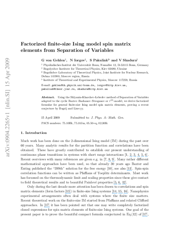
 S. Pakuliak
 Nikolai Iorgov