Object Recognition and Full Pose Registration from a Single Image for Robotic Manipulation Alvaro Collet Dmitry Berenson Siddhartha S. Srinivasa Dave Ferguson Abstract— Robust perception is a vital capability for robotic manipulation in unstructured scenes. In this context, full pose estimation of relevant objects in a scene is a critical step towards the introduction of robots into household environments. In this paper, we present an approach for building metric 3D models of objects using local descriptors from several images. Each model is optimized to fit a set of calibrated training images, thus obtaining the best possible alignment between the 3D model and the real object. Given a new test image, we match the local descriptors to our stored models online, using a novel combination of the RANSAC and Mean Shift algorithms to register multiple instances of each object. A robust initialization step allows for arbitrary rotation, translation and scaling of objects in the test images. The resulting system provides markerless 6-DOF pose estimation for complex objects in cluttered scenes. We provide experimental results demonstrating orientation and translation accuracy, as well a physical implementation of the pose output being used by an autonomous robot to perform grasping in highly cluttered scenes. I. I NTRODUCTION Autonomous robots operating in human environments present some extremely challenging research topics in path planning and dynamic perception, among others. Whether it is in the workplace or in a household, a common characteristic is the lack of static surroundings: people walk around, tables and chairs are moved, objects are left in different places. In order to successfully navigate in, and interact with, such an environment, accurate and robust dynamic perception is a must. In particular, an object recognition system that provides accurate 6-DOF pose is very important for performing complex manipulation tasks. The object recognition and registration system we propose handles arbitrarily complex non-planar objects, is fully automatic and based on natural (marker-free) features of a single image. It is robust to outliers, partial occlusions, changes in illumination, scale and rotation. It is able to detect multiple objects and multiple instances of the same object in a single image, and provide accurate pose estimation for every instance. Using a calibrated camera, it is able to localize each object in the robot’s coordinate frame to enable on-line manipulation, as shown in Fig. 1. Our system takes the core algorithm of Gordon and Lowe [1] and extends it with a model alignment step that enables accurate localization (section III-B), an automatic A. Collet and D. Berenson are with The Robotics Institute, Carnegie Mellon University, 5000 Forbes Ave., Pittsburgh, PA - 15213, USA. {acollet, dberenson}@cs.cmu.edu S. Srinivasa and D. 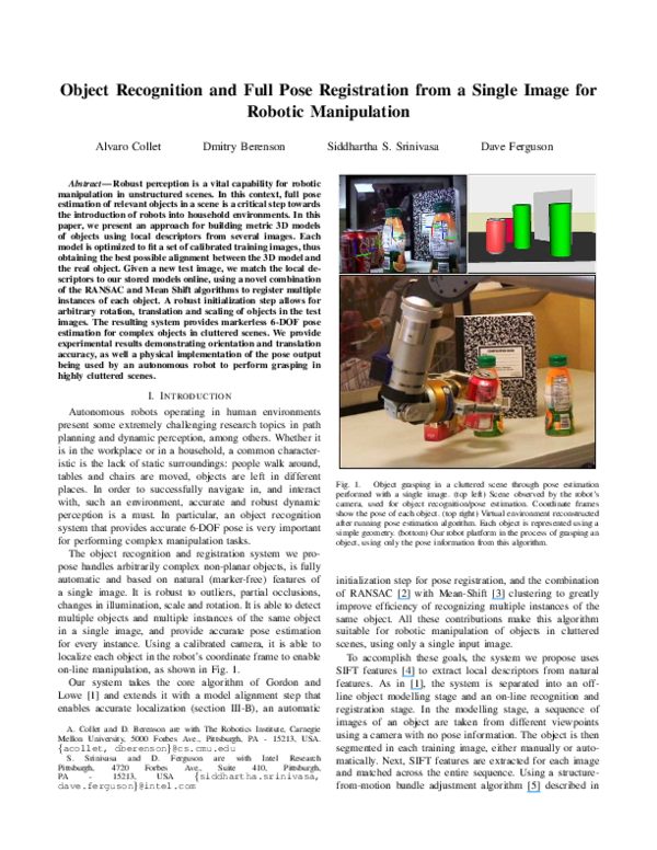Ferguson are with Intel Research Pittsburgh, 4720 Forbes Ave., Suite 410, Pittsburgh, PA 15213, USA {siddhartha.srinivasa, dave.ferguson}@intel.com Fig. 1. Object grasping in a cluttered scene through pose estimation performed with a single image. (top left) Scene observed by the robot’s camera, used for object recognition/pose estimation. Coordinate frames show the pose of each object. (top right) Virtual environment reconstructed after running pose estimation algorithm. Each object is represented using a simple geometry. (bottom) Our robot platform in the process of grasping an object, using only the pose information from this algorithm. initialization step for pose registration, and the combination of RANSAC [2] with Mean-Shift [3] clustering to greatly improve efficiency of recognizing multiple instances of the same object. All these contributions make this algorithm suitable for robotic manipulation of objects in cluttered scenes, using only a single input image. To accomplish these goals, the system we propose uses SIFT features [4] to extract local descriptors from natural features. As in [1], the system is separated into an offline object modelling stage and an on-line recognition and registration stage. In the modelling stage, a sequence of images of an object are taken from different viewpoints using a camera with no pose information. The object is then segmented in each training image, either manually or automatically. Next, SIFT features are extracted for each image and matched across the entire sequence. Using a structurefrom-motion bundle adjustment algorithm [5] described in Section III, we obtain a metric 3D reconstruction of the desired object, as illustrated in Fig. 2. Finally, the 3D model is optimally aligned and scaled to accurately match a realistic representation of the object (Fig. 3). During the on-line stage described in Section IV, SIFT features for a new image are extracted and matched against those of each 3D model. For each object, Mean Shift clustering is applied to the SIFT keypoint 2D positions to group points belonging to the same object instance. On each cluster, RANSAC is combined with a Levenberg-Marquardt non-linear optimization step to recognize and register multiple instances of the object of interest. Finally, results from all clusters are merged together, removing multiple detections of the same object in different clusters (see Fig.6). The novelty of our approach is its ability to perform accurate 6D pose estimation of many objects in cluttered scenes, in an on-line fashion. The learned model alignment provides great accuracy without adding computational cost. The pose initialization (see Fig. 4) is robust to any transformation within the learned model space, enabling a fully automated system. Finally, the combination of RANSAC and Mean Shift clustering allows for efficient search of multiple instances of the same object with minimal extra overhead. II. R ELATED W ORK Reliable object recognition, pose estimation and tracking are critical tasks in robotic manipulation [6], [7], [8], [9] and augmented reality applications [10], [1]. While the range of techniques proposed for these purposes is vast, not many of them provide fully automated systems; most of the approaches developed for these tasks rely on overly simple initialization steps [11], cumbersome manual pose initialization procedures [12], or do not consider the issue at all [9]. In augmented reality research, the focus is obtaining the camera position and orientation with respect to an object or scene, and accurately registering the camera movement from one frame to the next. The well known AR toolkit [13] provides robust, accurate registration data from an object without any manual initialization. However, it needs to use markers for tracking, which makes it unsuitable for tracking multiple objects independently, and would require placing markers on each object the robot interacts with. Lepetit et al. [10] overcome the marker limitation by using CAD models of the tracked objects/scenes, and precomputing keyframes from the most informatives views of each scene. Gordon and Lowe [1] present the algorithm on which this paper is based, providing a method for accurate camera tracking using learned models of a scene and SIFT features, but no quantitative localization/orientation results are shown. In general, the main difficulty when evaluating our method against the aforementioned articles is the lack of comparable results: while augmented reality research focuses on minimizing camera jitter and drift, we wish to obtain accurate localization and orientation of objects in the real world. In robotics research, many approaches try to solve a simplified pose estimation problem, in which the object is Fig. 2. Learning sparse 3D models. (a-b) Training images for a soda can and learned 3D model and camera positions. (c-f) Learned models for soda can (c), rice box (d), juice bottle (e) and notebook (f). Each box (c-f) contains an image of the object, a projection of its corresponding sparse 3D model, and its virtual representation in the robot’s workspace. usually assumed to be lying on a planar surface, hence restricting the search to a position [x y] plus an angular orientation [14], [15]. A more sophisticated method developed by Ekvall et al. [7], uses color co-occurrence histograms and geometric modeling to estimate the 6-DOF pose of objects. While the authors provide a fully automated system, this approach has several limitations: the algorithm is very sensitive to color variations; histogram-based methods make the recognition of several close instances of an object extremely hard; and geometric models rely on lines and edges for accurate localization, thus restricting the range of usable objects. Mittrapiyanuruk et al. [9] use Active Appearance Models (AAMs) to estimate the 6-DOF pose of objects. The authors provide similar results to our approach (less than 10mm of localization accuracy), although this method suffers from the known issues in AAMs, namely their troublesome initialization step and sensitivity to occlusions. Hinterstoisser et al.[16] propose the creation of sets of close feature points with distinctive properties to serve as natural 3D markers (N3Ms). Unfortunately, the authors only provide pass/fail experiments in synthetic images. It would be interesting to compare their performance and accuracy in real data. III. M ODELLING OBJECTS USING NATURAL FEATURES The first task towards the creation of our automated recognition and registration system is the training stage. While other approaches require objects with particular geometric properties (i.e. planar surfaces), need CAD models, or rely on the use of markers, our system uses natural features of the object to create a 3D metric model. Reliable local descriptors are extracted from natural features using SIFT [4]. SIFT features have proven to be one of the most distinctive and robust local descriptors across a wide range of transformations [17]. Matching between SIFT descriptors is performed using the Best Bin First [18] algorithm. Using structure from motion on the matched SIFT keypoints, we merge the information from each training image into a sparse 3D model. Finally, proper alignment and scale for each model are optimized to match the real object dimensions. A. Sparse 3D models In order to create a 3D model of an object, we first need to capture a set of training images of the object from various positions (see Fig. 2). To simplify this training stage, an ordered dataset is assumed, in which the most similar images to a given image are its peers. SIFT features are extracted from each image, and its descriptors are matched against those of its peer images. Pair-wise correspondences are then filtered by estimating the Fundamental matrix and enforcing the epipolar constraint on each pair of images [19]. Finally, multi-view correspondences are obtained by matching each set of pair-wise correspondences against all other sets. Each multi-view correspondence has one assigned SIFT feature, which can be either chosen from the set of matching SIFT features for that multi-view correspondence, or computed through clustering. In essence, multi-view correspondences are 2D projections of the 3D points of the object. Formally, T the relationship between a 3D point Pj = [Xj Yj Zj 1] T and its 2D projection in image i, pij = [xij yij 1] , can be expressed as: ≡ KTi Pj   R i ti = 0 1 pij Ti (1) (2) where K is a 3 × 3 intrinsic camera calibration matrix, and Ti is the camera transform comprised of Ri and ti , the rotation and translation of camera i, respectively. The symbol ≡ denotes an equality up to scale. A bundle adjustment algorithm [5] is used to build a sparse 3D model of an object from its multi-view correspondences. This algorithm jointly optimizes all 3D points Pj and extrinsic camera parameters Ri and ti , by minimizing the sum of reprojection errors of each 3D point into each image (see Eq. 4). It is noteworthy to mention that, while the intrinsic camera matrix K can also be optimized using this method, the reconstructed 3D models significantly decrease their localization accuracy. Therefore, it is advisable to obtain a better estimation of such parameters using a checkerboard calibration step. For a set of parameters P = [P1 · · · PN ] , R = [R1 · · · RM ] , t = [t1 · · · tM ] containing N 3D points and M camera positions, the optimal set of parameters (P∗ , R∗ , t∗ ) is given by score(P, Ri , ti ) = N X 2 [pij − proj(Pj , Ri , ti )] (3) j=1 (P∗ , R∗ , t∗ ) = arg min P,R,t M X score(P, Ri , ti ) (4) i=1 where proj() represents the non-linear perspective projection Fig. 3. Learning accurate model alignment. (right) input image. (left) Transformation Ta,1 corresponds to the original model without realignment. Ta,2 is the proper learned transformation Ta = [sRa |ta ]. Ta,3 corresponds to a model with proper orientation but double scale. function given by  u v  = proj(Pj , Ri , ti ) (5)       x u x/w  y  = K [Ri | ti ] Pj (6) = v y/w w The optimal set of parameters can be obtained with any generic non-linear minimization method, such as LevenbergMarquardt [20]. Gordon and Lowe [1] demonstrated that the convergence region for this problem is very broad. Therefore, a simple initialization approach such as placing all points in the XY plane and all cameras in the same arbitrary position, facing the XY plane, is sufficient to obtain accurate parameters after convergence. B. Model alignment with real-world objects The output model after bundle adjustment consists of a set P of N 3D points with their corresponding SIFT features, and a set R, t of M camera positions. While this model is already usable for object tracking, it requires one further alignment Ra , ta with the (manually set) coordinate frame of the real-world object, as well as a scaling s to match its size. The pose estimation algorithm computes the rotation and translation Rest , test of a model with respect to the camera frame. The projection of a 3D point in the real world onto a 2D point in an image is given by   sRa ta Pj (7) pj ≡ KTest 0 1 The transformation [sRa | ta ] can be obtained from a small sample of images with known ground truth Rgt , tgt by optimizing the following objective function   X sRa ta i i k (8) score(Ra , ta , s) = kTgt − Test 0 1 i for some norm on transformations. For our problem, we parametrize Ra by elements in S3 using its roll, pitch, and yaw, and ta by elements in R3 , and use the Euclidean norm in S3 × R3 in the optimization. Once a suitable [sRa | ta ] is found, it is used to build the final model with 3D points P′ :   sRa ta ′ Pj (9) Pj = 0 1 Fig. 4. Initialization steps for a subset of 6 correspondences. Red crosses refer to SIFT features in the input image, and blue circles refers to the 2D projections of the matching SIFT features in the 3D model. (a) Input image. (b) Training image with most common matches with input image. (c) Initial object pose, corresponds to that of the training image. (d) Scaling adjustment. (e) Rotation adjustment. (f) Translation adjustment. After these adjustments, the estimation is accurate enough to be given to the non-linear minimization procedure. IV. AUTOMATIC FULL POSE ESTIMATION The on-line stage of this system is a fully automated object recognition and pose estimation algorithm from a single image. Using the information from each sparse 3D model in section III, this algorithm is able to detect several objects and several instances of each object by combining the LM optimization with clustering and robust matching. The output information is the object types and their transformations Rest , test with respect to the camera frame. If the camera has been extrinsically calibrated, all objects can be accurately positioned in any virtual environment we wish to use (see Fig. 6). Each object is processed independently in each image when using this algorithm. Therefore, we will focus on the recognition and estimation of a single object type in this section. A. Initialization An accurate pose initialization is necessary to set the non-linear minimization procedure in its convergence region. After matching the test image against a 3D model’s SIFT descriptors, a correspondence list pi ↔ Pi is obtained. The training image with the most correspondences could be used as an initial rough estimation R1 , t1 of the object’s pose. Unfortunately, SIFT features are specifically designed to be invariant to scaling, translation, and orientation, thus providing a matching training image that may greatly differ from our test image. For example, the best feature match for the test image Fig. 4(a) is the training image Fig. 4(b). However, the non-linear optimization step cannot deal with such large differences. There exist several approaches to perform this initialization, which can be interpreted as a variants of the PnP problem. Many solutions have been proposed in the literature to obtain the position and orientation of a camera given a set of 2D ↔ 3D correspondences, such as POSIT[21], Clamped DLT and ePnP[22], among others. Alternatively, the Hough transform[23], [24] can be used to identify clusters of features in pose space that present a consistent orientation and translation. This prediction, however, could potentially have large errors due to perspective changes. In this section, we provide a simple yet robust alternative for initializing an object’s 3D model, whose main advantage over the aforementioned methods is its much greater speed. Our initialization uses a simple variant of the Orthogonal Procrustes Decomposition [25] that accounts for scaling. We first define pvi to be a 2D point in the test image, and ppj = proj(Pj , R, t) to be the 2D projection of the 3D point Pj onto the camera positioned at R, t. We first perform a scale correction using the standard deviation ratio of all pairwise distances within the two images pv and pp to displace the object closer or further away in the camera frame (z coordinate): v v u u N N u1 X u1 X
2 2 t v v (pi − p̄ ) σp = t ppj − p̄p (10) σv = N i=1 N j=1   tx,1 t′ =  ty,1  ppj = proj (Pj , R1 , t′ ) (11) σp σv tz,1 To perform the rotation initialization, we need to distinguish between out-of-plane and in-plane rotation. Outof-plane rotation modifies the object’s shape and visible area, whereas in-plane rotation does not (see Fig. 5). We have no information in the SIFT features that can help us correct errors in out-of-plane rotation. To correct in-plane rotation, we apply the solution to the Orthogonal Procrustes Decomposition, namely the alignment of pv and pp with its principal component: uv = PCA(pv ) up = PCA(pp )
θ = arccos uTv up   cos(θ) − sin(θ) 0 R′ =  sin(θ) cos(θ) 0  R1 0 0 1 ppi = proj (Pj , R′ , t′ ) (12) (13) (14) (15) This provides the rotation matrix R′ that minimizes the squared transformation error. Finally, the initial translation needs to be addressed. Given that the system needs to be robust to occlusions, it is unrealistic to set the object’s center at the average of pv . Instead, we must ensure that µv , µp , i.e. the averages of pv and pp , are at the same relative position from the projected model center C = [x y 1]T . Therefore, the model center computation is as follows: PN PN (16) µp = N1 i=1 ppi µv = N1 i=1 pvi
T ′ ′ C = proj [0 0 0 1] , R , t (17) ′ b −1 ′ C = µv − µp + C C =K C (18)  b ′  Cx tz t′′ =  Cyb t′z  (19) t′z Fig. 5. Examples of the different experiments run on the accuracy test. (Top row) Coke can translation test. (Middle row) Juice bottle out-of-plane rotation test. (Bottom row) Notebook in-plane rotation test. where C b represents the model center back-projected in 3-space. Finally, a robust initialization for the non-linear minimization procedure is Rinit = R′ , tinit = t′′ . B. Pose estimation of a single instance The objective of this algorithm is to obtain an optimal transformation R, t of a 3D model w.r.t. the camera frame. This can be accomplished with a non-linear minimization on the sum of reprojection errors between the projected 3D points from the model and the set of 2D points in the test image, pv . The optimal parameters R∗ , t∗ are defined as: min (R∗ , t∗ ) =arg R,t N X 2 [pvi − proj (Pi , R, t)] (20) i=1 The Levenberg-Marquardt non-linear minimization algorithm with initialization parameters Rinit , tinit provides an accurate solution for most cases in which only one object instance is present. C. Pose estimation of multiple instances One of the most important aspects of our algorithm is its ability to find multiple instances of the same object. We have integrated the recognition and pose estimation of multiple instances in the same iterative algorithm. The set of matched SIFT points pi ↔ Pi contains correspondences between an object type and a 3D model. However, those matched points can potentially belong to more than one instance, with no a priori way to detect this outcome. While a naı̈ve application of RANSAC alone should be enough to find all instances of an object in an image, the probability of finding a subset of points that all belong to the same object decreases exponentially with the number of instances present in an image. In turn, the required computation time grows exponentially, making this approach infeasible. However, the combination of RANSAC with a clustering technique avoids the exponential computation time increase, because closer points are more likely to be part of the same object instance (see Fig. 6 for details). In Fig. 6.b we see an image with 9 notebooks. Let us assume all notebooks have the same amount of correspondences, 30% of outliers, and that we require 5 inliers for a successful detection. According to RANSAC’s iterations estimation, finding one particular instance of a notebook with 95% probability requires over 1M iterations. On the other hand, clustering the correspondences in smaller sets as in Fig. 6.d means that fewer notebooks (at most 3) are present in a given cluster. In such a scenario, finding one particular instance of a notebook with 95% probability requires 16, 586 and 4386 iterations when 1, 2 and 3 notebooks, resp., are present in a cluster, at least three orders of magnitude lower than before. In our system, Mean Shift clustering is a good choice because no fixed number of clusters needs to be specified. The full algorithm is as follows: 1) Cluster SIFT feature 2D locations p using Mean Shift algorithm. Each cluster contains a subset of points pk . 2) For each cluster of points pk , choose a subset of n points and estimate a hypothesis with the best pose according to those points. If the amount of points consistent with the hypothesis is higher than a threshold ǫ, create a new object instance and refine the estimated pose using all consistent points in the optimization. Keep repeating this procedure until the amount of unallocated points is lower than a threshold, or the maximum number of iterations has been exceeded. 3) Merge all found instances from different clusters whose estimated R, t are similar. The instances with the most consistent points survive. V. E XPERIMENTS In order to prove our pose estimation algorithm’s suitability for robotic manipulation, two sets of experiments have been conducted. The first set evaluates our algorithm’s accuracy in estimating the position and orientation of objects in images. The second set uses the full pose estimation algorithm alongside a state-of-the-art planning algorithm to grasp objects with a Barrett WAM robotic arm. It is important to mention that in all experiments we have estimated the Fig. 6. The importance of clustering in cluttered scenes. The camera position is represented as a red and white pyramid. (Col 1) Scene with 1 soda can, 2 juice bottles and 3 notebooks. The water bottle is not an object in the database, and is therefore only treated as another occlusion. Note that the notebook on the right is upside down, and correctly detected. Without Mean Shift, this scene requires 121 iterations of RANSAC. With Mean Shift, it requires 38. (Col 2) Scene with 9 highly-occluded notebooks. Without Mean Shift, the algorithm is only able to find 6 notebooks before the 3000 iterations limit is reached. With Mean Shift, 9 clusters are formed and all 9 notebooks are detected -with no outliers- after 454 iterations. (Col 3) Scene with 2 soda cans, 2 juice bottles and 1 rice box. Without Mean Shift, 115 iterations. With Mean Shift, 33 iterations. (Col 4) Clusters of correspondences in Notebooks image. full 6-DOF pose of objects, and no assumptions were made on their orientation or position. In all cases, our algorithm clusters the scene with a Mean Shift radius of 100 pixels, and chooses subsets of 4 correspondences to compute each RANSAC hypothesis. The current system is implemented in Matlab, speeding up the most expensive computations (SIFT matching, Levenberg-Marquardt optimization) in C/C++. One dedicated computer is used to compute SIFT descriptors, and a second computer performs the actual recognition and pose estimation. Using the aforementioned parameters and setup, the average computation time ranges from 3 to 6 frames per second. A. Pose estimation accuracy In this set of experiments, we evaluate our algorithm’s accuracy over the short-to-medium distance most useful in robotic manipulation. All experiments have been conducted on a table on which a camera has been fixed and extrinsically calibrated. The coordinate origin is set to be the table’s corner. Four common objects with different shapes and sizes were used: a juice bottle, a coke can, a rice box and a notebook. Given the randomized nature of our implementation, 10 images are taken at each test position and their results averaged, as shown in Fig. 7, to obtain a reliable measure of accuracy. Fig. 5 depicts some examples of images used in the pose estimation accuracy test. 1) Translation: The first experiment measures the pose estimation accuracy of each object in the 30 to 90 cm distance range. Each object is placed alone in an image and moved in 10 cm intervals, from 30 to 90 cm away from the camera (depth test) and laterally from 0 to 20 cm. Table I shows the average translation error (in cm) for each object and distance, measured as the Euclidean distance between the center of the estimated object and the center of the ground truth object. Best results are obtained in the 40-70cm range, but it is remarkable that the average error across all objects TABLE I T RANSLATION ERROR TEST. A LL DISTANCES IN CM . Distance from camera (cm) 30 40 50 60 70 80 90 Can 0.93 0.14 0.61 0.55 – – – Juice 0.55 0.82 0.63 0.94 0.41 0.81 2.56 Rice 0.47 0.34 0.24 0.49 0.49 0.98 1.36 Notebook 0.98 0.75 0.51 0.36 0.49 0.75 0.95 and distances is only 0.67cm. No results are shown for the Coke can in the furthest distances because the algorithm does not find enough features to determine its pose accurately. 2) Out-of-plane rotation: The out-of-plane rotation test measures the orientation accuracy of our algorithm for a fixed depth. Keeping the object’s center at 50 cm away from the camera, each object is rotated with respect to the Z axis from -45 to 45 degrees, in 15 degree intervals. Orientation error for a given axis v is computed as the angle between that axis in Fig. 7. (left) Distribution of translation error (all objects). Average error: 0.67 cm. (right) Distribution of all rotation errors. Average error: 3.81 degrees. Fig. 8. Examples of grasping objects in cluttered scenes. The first four images (top row, plus bottom-left) show our robotic arm grasping a soda can, bottle juice, rice box and notebook (resp.). The fifth image (bottom-center) shows a detail of the required position accuracy necessary for cluttered scenes: the arm executes a trajectory that passes less than 1 cm away from a soda can and a rice box without touching them. The bottom-right image shows our whole test environment while the robot manipulates a rice box. TABLE II O UT- OF - PLANE ROTATION ERROR . A LL ERRORS IN DEGREES . Angle (degrees) −45 −30 −15 0 15 30 45 Can 10.71 6.03 3.35 0.88 1.82 4.80 6.27 Juice 4.46 2.50 2.17 1.38 2.15 2.53 9.31 Rice 0.97 0.71 0.47 0.11 2.38 3.67 3.41 TABLE III I N - PLANE ROTATION ERROR . A LL ERRORS IN DEGREES . Notebook 1.14 1.08 0.87 0.06 2.13 2.05 3.04 Angle (degrees) −45 −30 −15 0 15 30 45 the estimated solution and its ground truth counterpart, i.e.: uest = Rest v ugt = Rgt v kuTest ugt k ), θ = arccos( kuest kkugt k (21) (22) where Rest and Rgt are the estimated and ground truth 3 × 3 rotation matrices, respectively, and v is a column 3-vector that represents one of the axes. Table II shows the out-ofplane rotation error results. The average out-of-plane rotation error is 3.81 degrees. It is noteworthy to mention that the soda can and the juice bottle obtain the poorest results at −45 and 45 degrees, respectively, because these are the views with lowest density of SIFT features in their 3D models. Even in these extreme cases, such errors proved to be small enough for most of our grasping experiments. 3) In-plane rotation: The in-plane rotation test measures the orientation accuracy of our algorithm on 2D rotations parallel to the image plane. For a given depth (50cm) and position, each object is tilted up to 45 degrees to each side in 15 degree intervals. Table III shows the in-plane rotation error results. The average in-plane rotation error is 1.23 degrees. Can 4.81 4.25 2.57 1.02 0.42 1.22 2.76 Juice 1.75 1.29 0.96 1.59 0.99 0.48 1.05 Rice 1.02 0.74 0.16 0.51 0.58 0.11 0.34 Notebook 0.54 0.62 1.94 1.24 0.03 1.02 0.94 B. Grasping objects To gauge the effectiveness of our object pose estimation approach for manipulation, we integrated the approach with a planning algorithm for the Barrett WAM arm. The planning algorithm, called the Inverse-Kinematics BiDirectional Rapidly-exploring Random Tree algorithm (IKBiRRT) [26], plans a trajectory for the arm starting from its current configuration and ending at a configuration that places the wrist of the robot at an acceptable location for grasping. Each object that was localized has an associated set of wrist locations that are acceptable for grasping. Once the transform of the object is found, the associated wrist locations are input as goal regions for the planner, which then samples from these goal regions as it plans. Note that, for scenes where multiple graspable objects are present, we input all the associated wrist locations for all objects into the planner, which finds a trajectory to reach any one of them. Once the robot completes the trajectory, the fingers are closed and the object is lifted. Snapshots from the experiments are show in Fig. 8. Notice that the accuracy of the pose estimates are good enough for the robot to squeeze into narrow openings and pick up objects within the clutter. The grasping tests were performed by placing a single object on a table within the robot’s reachable space. Prior to TABLE IV G RASPING TEST Attempts Successful grasps Can 25 22 Juice 25 25 Rice 25 21 Notebook 25 23 Total 100 91 each grasping attempt, the object is placed in a new arbitrary position and orientation (standing up, sideways and upside down). As seen in IV, our results show an impressive 91% overall grasping success rate, thus confirming the statement that our pose estimation algorithm is accurate enough to enable robotic manipulation of the detected objects. A video containing vision-based grasping experiments in cluttered scenes is submitted alongside this paper. VI. C ONCLUSIONS AND F UTURE W ORK We have presented and validated a system for the markerless recognition and registration of common household objects. A strength of our current algorithm is that it provides full pose even from just one image. We have demonstrated that the results are accurate enough for a robot to reach into a cluttered scene registered from just one image and pick up all of the objects. We are currently exploring two extensions: the integration of pose estimates from multiple views, and active sensing to move the arm to good views for pose estimation. We believe that our system provides a crucial capability that will enable mobile manipulators to function and interact in crowded indoor environments. VII. ACKNOWLEDGMENTS This material is based upon work partially supported by the National Science Foundation under Grant No. EEC0540865. Alvaro Collet is partially supported by La Caixa fellowship. Special thanks to Christopher G. Atkeson for his insightful comments and discussions. R EFERENCES [1] I. Gordon and D. G. Lowe, “What and where: 3d object recognition with accurate pose,” in Toward Category-Level Object Recognition, ser. Lecture Notes in Computer Science, J. Ponce, M. Hebert, C. Schmid, and A. Zisserman, Eds., vol. 4170. Springer, 2006, pp. 67–82. [2] M. A. Fischler and R. C. Bolles, “Random sample consensus: a paradigm for model fitting with applications to image analysis and automated cartography,” Commun. ACM, vol. 24, no. 6, pp. 381–395, June 1981. [Online]. Available: http://dx.doi.org/10.1145/358669.358692 [3] Y. Cheng, “Mean shift, mode seeking, and clustering,” IEEE Transactions on Pattern Analysis & Machine Intelligence, vol. 17, no. 8, pp. 790–799, 1995. [4] D. G. Lowe, “Distinctive image features from scale-invariant keypoints,” International Journal of Computer Vision, vol. 60, pp. 91–110, 2004. [5] R. Szeliski and S. B. Kang, “Recovering 3d shape and motion from image streams using non-linear least squares,” Robotics Institute, Carnegie Mellon University, Pittsburgh, PA, Tech. Rep., March 1993. [6] G. Taylor and L. Kleeman, “Fusion of multimodal visual cues for modelbased object tracking,” in In Australasian Conference on Robotics and Automation (ACRA2003), Brisbane,Australia, 2003. [7] S. Ekvall, D. Kragic, and F. Hoffmann, “Object recognition and pose estimation using color cooccurrence histograms and geometric modeling,” Image Vision Comput., vol. 23, no. 11, pp. 943–955, 2005. [8] S. Zickler and M. Veloso, “Detection and localization of multiple objects,” Humanoid Robots, 2006 6th IEEE-RAS International Conference on, pp. 20–25, Dec. 2006. [9] P. Mittrapiyanuruk, G. N. DeSouza, and A. C. Kak, “Calculating the 3d-pose of rigid-objects using active appearance models.” in IEEE International Conference on Robotics and Automation. IEEE, 2004, pp. 5147–5152. [10] L. Vacchetti, V. Lepetit, and P. Fua, “Stable real-time 3d tracking using online and offline information,” IEEE Transactions on Pattern Analysis and Machine Intelligence, vol. 26, no. 10, pp. 1385–1391, 2004. [11] M. Vincze, M. Ayromlou, W. Ponweiser, and M. Zillich, “Edgeprojected integration of image and model cues for robust model-based object tracking,” I. J. Robotic Res., vol. 20, no. 7, pp. 533–552, 2001. [12] V. Gengenbach, H.-H. Nagel, M. Tonko, and K. Schafer, “Automatic dismantling integrating optical flow into a machine vision-controlled robot system,” IEEE International Conference on Robotics and Automation, vol. 2, pp. 1320–1325 vol.2, Apr 1996. [13] H. Kato and M. Billinghurst, “Marker tracking and hmd calibration for a video-based augmented reality conferencing system,” in Proceedings of the 2nd International Workshop on Augmented Reality (IWAR 99), San Francisco, USA, Oct. 1999. [14] B. A. J. Walter, “Gabor filters for object localization and robot grasping,” in IEEE Proceedings of the International Conference on Pattern Recognition. Washington, DC, USA: IEEE Computer Society, 2000, p. 4124. [15] J. Zhang, R. Schmidt, and A. Knoll, “Appearance-based visual learning in a neuro-fuzzy model for fine-positioning of manipulators,” in IEEE International Conference on Robotics and Automation, 1999, pp. 1164–. [16] S. Hinterstoisser, S. Benhimane, and N. Navab, “N3m: Natural 3d markers for real-time object detection and pose estimation,” in IEEE International Conference on Computer Vision, 2007, pp. 1–7. [17] K. Mikolajczyk and C. Schmid, “A performance evaluation of local descriptors,” IEEE Transactions on Pattern Analysis & Machine Intelligence, vol. 27, no. 10, pp. 1615–1630, 2005. [Online]. Available: http://lear.inrialpes.fr/pubs/2005/MS05 [18] J. S. Beis and D. G. Lowe, “Shape indexing using approximate nearestneighbour search in high-dimensional spaces,” in In Proc. IEEE Conf. Comp. Vision Patt. Recog, 1997, pp. 1000–1006. [19] R. I. Hartley and A. Zisserman, Multiple View Geometry in Computer Vision, 2nd ed. Cambridge University Press, ISBN: 0521540518, 2004. [20] D. W. Marquardt, “An algorithm for least-squares estimation of nonlinear parameters,” SIAM Journal on Applied Mathematics, vol. 11, no. 2, pp. 431–441, 1963. [21] D. F. Dementhon and L. S. Davis, “Model-based object pose in 25 lines of code,” Int. J. Comput. Vision, vol. 15, no. 1-2, pp. 123–141, 1995. [22] V. Lepetit, F. Moreno-Noguer, and P. Fua, “Epnp: An accurate o(n) solution to the pnp problem,” Int. J. Comput. Vision, vol. 81, no. 2, pp. 155–166, 2009. [23] D. H. Ballard, “Generalizing the hough transform to detect arbitrary shapes,” Pattern Recognition, vol. 13, no. 2, pp. 111–122, 1981. [Online]. Available: http://dx.doi.org/10.1016/0031-3203(81)90009-1 [24] W. E. L. Grimson and D. P. Huttenlocher, “On the sensitivity of the hough transform for object recognition,” IEEE Trans. Pattern Anal. Mach. Intell., vol. 12, no. 3, pp. 255–274, 1990. [25] P. Schonemann, “A generalized solution of the orthogonal procrustes problem,” Psychometrika, vol. 31, no. 1–10, 1966. [26] D. Berenson, S. Srinivasa, D. Ferguson, A. Collet, and J. Kuffner, “Manipulation planning with workspace goal regions,” in IEEE Int’l Conf. on Robotics and Automation (ICRA’2009),Kobe,Japan, 2009.