Sonic Explorations of GumowskiMira Maps
Timothy S. H. Tan
Institute of Sonology
The Royal Conservatoire, The Hague
WLPEUHWDQ#JPDLOFRP
ABSTRACT
This paper studies the use of GumowskiMira maps for
sonic arts. GumowskiMira maps are a set of chaotic sys
tems that produce many organic orbits that resemble cells,
flowers and other life forms. This has prompted mathema
ticians and eventually artists to study them. These maps
carry a potential for use in the sonic arts, but until now
such use is nonexistent. The paper describes two ways of
using GumowskiMira maps: for synthesis and spatializa
tion. The synthesis approach, which runs in realtime,
takes the dynamical system output as the real and imagi
nary input to an inverse Fourier transformation, thus di
rectly sonifying the algorithm. The spatialization ap
proach uses the shapes of GumowskiMira maps as shapes
across the acoustic space, using the first 128 iterations of
each map as audio particles. The shapes can change based
on the maps’ initial parameters. The maps are explored in
live performance using Leap Motion and Cycling ’74’s
MIRA for iPad as control interfaces of audio processing in
SuperCollider. Examples are given in two works, Cells #1
and #2.
1.INTRODUCTION
The GumowskiMira map (henceforth called GM map)
was named after I. Gumowski and C. Mira, who were stud
ying various chaotic maps from the 1960s [1]. Around
1970, while at CERN, Gumowski was studying chaotic in
stability in accelerators and storage rings, and collaborated
with the Toulouse Research Group led by Mira [1, pp. 129
131]. What is now known as the GM map was based on a
dissipative perturbation of one such map studied by
Gumowski and then with Mira [1, pp. 121124]. It com
prises the following equations:
ݔାଵ ൌ ݕ ߙǤ ݕ Ǥ ሺͳ െ ߪǤ ݕଶ ሻ ܨሺݔ ሻ
ݕାଵ ൌ െݔ ܨሺݔାଵ ሻ
(1)
There are a few variants of GM maps. According to [1,
pp. 180184], two different F(x) exist:
ଶ
ܨሺݔሻ ൌ ߤǤ ݔ ሺͳ െ ߤሻǤ ݔǤ ݁
ܨሺݔሻ ൌ ߤǤ ݔ
ଶǤሺଵିఓሻǤ௫ మ
ଵା௫ మ
భషೣమ
ర
(2)
(3)
Copyright: © 2017 Timothy S. H. Tan and PerMagnus Lindborg. This is
an openaccess article distributed under the terms of the Creative
Commons Attribution License 3.0 Unported, which permits unrestricted
use, distribution, and reproduction in any medium, provided the original
author and source are credited.
H EA RING THE S E LF
PerMagnus Lindborg
School of Art, Design and Media
Nanyang Technological University
SHUPDJQXV#QWXHGXVJ
The equation (1) also appears in a slightly different form
in [1, pp. 179], with F(x) is similar to (3):
ݔାଵ ൌ ݕ ߙǤ ݕ Ǥ ሺͳ െ ߪǤ ሺݕଶ ͵Ǥ ݔଶ ሻሻ ܨሺݔ ሻ
ݕାଵ ൌ െݔ ܨሺݔାଵ ሻ
(4)
ܨሺݔሻ ൌ ߤǤ ݔ
ଶǤሺଵିఓሻǤ௫ మ
ଵା௫ ర
(5)
These variations can produce similar shapes, albeit with
slightly different ranges of usable initial parameters.
GM maps have some benefits not found in other chaotic
systems. Across the phase space, GM maps can produce
intricate, organic images that resemble cells, flowers and
other lifeforms. These images can vary a lot in shapes, and
often possess different rotational or reflection symmetries.
Whereas a number of mathematicians [2] and artists [3]
have studied GM maps in detail, until now nobody has
used these maps as sonic parameters. Besides, GM maps
are still less wellknown than other chaotic systems such
as the logistic map, Chua circuit, Rössler attractor and
double pendula. After all, chaotic systems have been used
to map onto frequencies [4, 5], rhythm and note durations
[4], dynamic levels (velocities) [5], timbre [6, 7], grain fre
quencies [6] and grain lengths [7]. Even SuperCollider [8]
has many chaotic UGens that generate sounds based on
audiorate calculations of chaotic systems, such as
LinCongN and GbmanTrig.
This article presents how the two authors have used GM
maps for synthesis and spatialization, with their methodol
ogies, results and discussions.
2.GM MAPS FOR SYNTHESIS
Lindborg developed a program in Max [9] for concurrent
realtime synthesis and visualization of a GM map. The
state of the GM map is updated for each audio sample (Fig
ure 1) and its output (x, y) is mapped to the real and imag
inary input of an inverse Fourier transform (Figure 2).
Used as an experimental audio synthesizer, the output
has been employed in two sonic artworks in the past year
[10] [11].
As pointed out by Dean et al. [12], the concurrent audio
visual output of the system correspond fully on a synthesis
level but this does not necessarily mean that they corre
spond perceptually. Future work aims to evaluate experi
mentally the extent to which auditory and visual modalities
of the outputs correspond.
195
acoustic space. They also easily broach the “conflict / co
existence” behavioral relationship addressed by Smalley
[21]: Tiny changes to initial parameters create small errors
that accumulate and later cause great deviations to the or
bits. These orbits can conflict and even tangle each other.
Figure 1. Max implementation of the dynamical system
feedback.
Figure 2. Max implementation of the GM map’s twodi
mensional output as input to an inverse Fourier transform.
3.GM MAPS FOR SPATIALIZATION
To date, chaos has been applied to spatialization in [13]
and fractals in [14], but for algorithmic spatialization, there
has been some progress. Some have implemented algorith
mic spatialization with OpenMusic, as in [14]–[16],
whereas Schacher et al. have composed with swarm algo
rithms and flocking, both controlling spatialization among
other parameters [17]. Lindborg has utilized particle colli
sions registered in bubble chamber images [18] as well as
the collision of particles [19] for algorithmic spatialization.
Using GM maps for spatialization can prove interesting
and innovative. The numerous patterns of GM maps tend
to be highly distinctive and thus can provide equally dis
tinctive spatial shapes across the acoustic space. The
shapes also change unpredictably and very quickly even if
there are tiny changes to the initial parameters. For Tan,
this meant a vast choreography of spatial shapes. In fact,
Deleuze and Guattari, while discussing philosophy, had
even reflected on the speed at which these shapes change:
Chaos is not so much defined by its disorder
as by the infinite speed with which every
form taking shape in it vanishes. It is a void
that is not a nothingness but a virtual, con
taining all possible particles and drawing out
all possible forms, which spring up only to
disappear immediately, without consistency
or reference, without consequence. Chaos is
an infinite speed of birth and disappearance
[20].
Their last point makes spatializing chaotic maps like GM
maps a highly efficient tool in building up tension and in
tensity, furthermore engaging listeners through a given
196
Moreover, using chaotic maps for spatialization is more
robust than for other parameters. When other parameters
rely on streams of numerical outputs, the heard results of
ten correspond poorly with the original map used. For in
stance, the timbres of the gingerbread man map in
GbmanTrig from SuperCollider may sound interesting, but
listeners cannot identify its timbre specifically with
GbmanTrig. Besides, scaling, rotation, translation and
skewing of these maps easily preserves their visual percep
tion, but distorts their listening experience when heard as
streams of output. On the other hand, spatialization of cha
otic maps rely on graphical representations of these maps,
thereby preserving the shapes across the acoustic space.
Because GM maps can create captivating visual shapes,
Tan has focused on recreating these shapes through spati
alization of GM maps in the acoustic space.
3.1 Implementation
When chaotic maps exhibit their sensitivity to initial con
ditions, they imply the need to compare between close
neighboring values of initial parameters. Plotting the di
vergent orbits one iteration at a time inadequately provides
a fuller picture of these maps, and worse still when the pre
vious iterations disappear as the sound travels along the
orbit. This makes the implication of comparison too long
and weak, thereby poorly demonstrating sensitivity to ini
tial conditions. Instead, Tan uses all the iterations of each
GM map as simultaneous audio particles for the acoustic
space, similar to Fonseca’s audio particle system in his
“Sound Particles” software [22] [23]. These iterations are
updated instantaneously whenever the initial parameters
change. Both methods easily highlight the comparisons
and preserve the picture of the maps, and thus the maps
can continue to demonstrate sensitivity to initial condi
tions.
One challenge is the need to balance between providing
an adequate image of the GM map and minimizing CPU
processing usage. As such, only 128 iterations per map are
used as audio particles, and only three GM maps are used.
Too many particles can overload the CPU and disrupt real
life performances involving GM maps.
Additionally, whenever the GM maps change their
shapes, the maps’ particles skip directly to their new posi
tions, without the need to consider the Doppler Effect. Un
like a particle system in which a particle can have a life of
its own, here the audio particles live and die together
whenever their respective maps are switched on or off.
A visualizer of the particle systems ensures that the per
former can see where the particles are; such a feature also
doubles as visuals for the audience to observe the particles’
positions and orbits. The size of the speaker space, which
2017 IC M C / EM W
covers the audiences in a concert hall, is similar to the size
of the visualizer, so as to maintain close correspondence
between audio and visuals. Audio particles can exceed the
boundaries of the visualizer and sound behind the speakers
(often more softly), so as not to overcrowd within the
speaker space. This allows better localization of the parti
cles (Figure 3).
Each GM map can be switched on or off. Usually only
one GM map starts the work, then is joined by the second,
and finally the third.
The range of iterations is confined within the first 128
iterations. This can be narrowed, so as to scrutinize the
movements of that number of particles. With modulo op
eration, the iteration index can be filtered with divisors of
17 and remainders of 06. At times where the GM maps
often look similar, this modulo filter reveals that the same
iteration index of each map occupies very different places
(Figure 4). As such, the modulo filter is often used to play
with the spatiality of the GM maps.
Figure 3. The visualizer of the particles’ positions based
on the three GM maps. Dashed square lines at the center
indicate the size of the speaker space, which in real life sur
rounds the audiences in a concert hall.
Not too many particles are allowed to crowd within the
speaker space, so as to make the spatial shape of the GM
maps clearer. Other than using three GM maps with a max
imum of 128 audio particles per map, secondorder 2D
Ambisonics is used. The spatial image of the GM maps can
be zoomed in and out, so as to reveal the intricate inner
shapes of the maps. The speaker setup, which surrounds
the audiences, is octophonic. This is used along with the
visualizer mentioned just above.
Figure 4. An instance of three GM maps played together
in Cells #2. Left: without modulo filter; right: with modulo
filter of divisor 4 and remainder 2.
The GM maps are performed with MIRA on iPad (with
Max 7) by Cycling ’74 [9], as well as Leap Motion [24]
(with Processing 3 [25]). These two interfaces enable the
performer to play with speed: MIRA for slow changes, and
Leap Motion for fast changes. Leap Motion communicates
with MIRA via Open Sound Control (OSC), and likewise
for MIRA with SuperCollider.
In order to differentiate which particles belong to which
GM map, each GM map has a different synth and thus tim
bre. This is to prevent all the audio particles from different
GM maps from blending together as if they are generated
from the same map. Normally one map contains some ad
ditive synthesis UGens, another some ChaosGens, and the
last granular synthesis. In turn, their particles have varying
parameters based not on their iteration index, but their po
sitions in space. The particles’ positions can affect the par
ticles’ frequencies and other audio effects. This is im
portant in varying the sounds of each particle, because if
the same sound is applied to every particle in a particle
system, it sounds almost similar to that sound used in one
particle whose size covers a far larger space (e.g. directly
from one speaker), thereby making the particle system use
less. For the visualizer, each GM map is assigned a color,
as a visual aid to differentiate the GM maps.
Leap Motion is very sensitive to the performer’s hand
positions. This fits well for performing chaotic works,
since chaotic systems are also sensitive to initial condi
tions, and accuracy is not so important in this context. This
enables the resultant shapes to transform quickly, but not
slowly, because it is difficult to control hand positions un
der Leap Motion’s high sensitivity. The hand parameters
are chosen and mapped based on ease and comfort. Only
the ranges of Į= [0.25, 0.25], ı= [0.25, 0.25], ȝ = [1.0,
1.0], x0 = [2.0, 2.0] and y0 = [2.0, 2.0] are used as the
initial parameters, as in these ranges, generally the maps
are conservative, do not enter infinity too soon, and do not
settle into a stable attractor at the origin within the first 128
iterations. The last feature tends to create an unwanted cen
tral ringing tone that overwhelms other audio particles.
The form is based on the rate of change of the initial pa
rameters. The music starts slowly, exploring and scrutiniz
ing the different spatial shapes of each map, before speed
ing up from the middle. Often the shapes are repeated at
the start, so that listeners can realize that they are not lis
tening to a random system, but a chaotic system of unpre
dictable, but specific shapes.
In contrast, MIRA allows the performer to play with one
or two parameters at a time on the iPad. This mode allows
better accuracy and slower changes than the Leap Motion
mode. One can switch between the MIRA mode and the
Leap Motion mode, in which only one of the two can affect
the parameters. For both cases, MIRA will track the
changes in the parameters as a visual feedback to the per
former. (MIRA also tracks the parameters changed by
Leap Motion through OSC.)
H EA RING THE S E LF
197
Figure 5. Three GM maps for Cells #1. Top: (1) with
(2) for F(x), middle: (1) with (3), bottom: (4) with (5).
Į = 0.03125, ı = 0.125, ȝ = 0.765625, x0 and y0 = 0.25,
and n = 128. Ranges of both axes are [12.5, 12.5].
198
Figure 6. Three GM maps for Cells #2, using (1) with (3)
for F(x), Į = 0.03125, ı = 0.125, x0 and y0 = 0.25, and
n = 128, but ȝtop = 0.765625, ȝmiddle = ȝtop + 212 and
ȝbottom = ȝtop + 211. Ranges of both axes are [12.5, 12.5].
2017 IC M C / EM W
3.2 &HOOVand&HOOV
Tan composed Cells #1 (2016, rev. 2017) and Cells #2
(2017) with Leap Motion and Max with MIRA for perfor
mance interface, and SuperCollider 3.8.0 for audio pro
cessing. Both works are to be performed live for a two
dimensional 8.1 speaker setup. Usually visuals of the GM
maps are projected to a large screen in front of the audi
ences, because GM maps remain unknown to many.
Cells #1 involves three GM maps, formed by coupling (2)
and (3) with (1), and (5) with (4), and using the first 128
iterations (Figure 5). Tan wants to study how the shapes
will look and sound if the same set of initial parameters to
these three maps is applied. Cells #2 also involves three
GM maps. This time, all three use the same equation (1),
with (3) for F(x), but the first and the second had ȝ that
differs by 212, and likewise for the second and third (Fig
ure 6). In both works, all these maps exist alongside each
other and contest for spatial prominence and likeness and
differences on their orbits in the same acoustic space. Both
works are meant for an octaphonic speaker setup with sec
ondorder Ambisonics, for greater spatial clarity.
3.3 Artistic Results
The spatial shapes can generally be identified, especially
by applying the modulo filter, but more work is needed to
make spatial shapes even clearer. The modulo filter and the
limit on the range of iterations work best for Cells #2, es
pecially when the maps often overlap each other but the
particles with the same iteration indices are at different or
even opposite places. Timbrewise, the chosen timbres for
each GM map remain distinct and do not blend, and this is
required. One listener had even highlighted the timbral va
riety of Cells #2. Additionally, some listeners had found
the performance with MIRA and Leap Motion very engag
ing, and noted the close correspondence between the
sounds and visuals. Meanwhile, Cells #1, originally com
posed in 2016, is now being revised to be on par with Cells
#2.
3.4 Discussion
Chaotic maps, such as GM maps, can be a powerful tool
for spatialization. However, it can be difficult trying to rep
licate the success of visualizing GM maps (or other chaotic
maps) across the audio spatial realm, when creative moti
vations conflict with technical constraints.
Attempts to produce complete shapes of GM maps au
rally with a lot of audio particles will cause overcrowding
inside the listening space, thus blurring the choreography
of the spatial shapes. As such, just the first 128 iterations
for one map are already adequate enough as audio parti
cles. Besides, having a lot of particles enhances and does
not blur the visual experience, but blurs and distorts the
listening experience. While visual particles do not diffuse
light themselves and blur their own shapes, audio particles
can at best only represent the ideal visual particle. Breg
man elaborates that:
H EA RING THE S E LF
This way of using sound has the effect, how
ever, of making acoustic events transparent;
they do not occlude energy from what lies
behind them. The auditory world is like the
visual world would be if all objects were
very, very transparent and glowed in sput
ters and starts by their own light, as well as
reflecting the light of their neighbors. This
would be hard world for the visual system to
deal with [26].
Despite efforts to reproduce the shapes of the GM maps
as faithfully as possible, the acoustic space has some re
strictions. One implication of Bregman’s is that while
anyone can replicate the directionality, scale and distribu
tion of particles across the space, the sharpness in the edges
and corners remains poorly defined. This can easily blur
the shapes’ intricate designs and corners, as well as cover
the holes in between the particles. As such, having thou
sands of audio particles like of visual particles do not en
hance the listening experience similarly to the visual expe
rience. By this approach, one can increase the number of
speakers for better spatial definition and clarity, though
perhaps not so costeffectively.
One drawback of performing with realtime audio parti
cle systems is that as the number of particles increase, both
the demand for audio processing power and the chance of
a breakdown also increase. Whereas visual implementa
tions of GM maps tend to involve hundreds or even thou
sands of particles, doing likewise for audio easily over
loads the CPU and thus handicaps reallife performances
of the works. Currently Fonseca’s “Sound Particles” soft
ware still cannot perform realtime rendering and play
back. Cells #2 went smoothly during rehearsals and sound
check, but halfway through the actual performance at the
Institute of Sonology, crashed just after the three GM maps
have been introduced. This was likely due to the audio in
terface (Focusrite Scarlett 18i20) unable to handle Super
Collider’s immense processing power, thereby causing the
audio interface to disconnect from SuperCollider. The per
formance had to be aborted. Work is underway reducing
CPU usage in one laptop, perhaps by splitting the pro
cessing power into more than one laptop and inviting one
extra performer, for both Cells.
While tempo is used to build form, listeners often per
ceive fast changes in spatial shapes as random instead of
being chaotic. These intricate shapes are hence no longer
perceived as specific to GM maps, even if they indeed are.
As such, the tempo will be reduced across both Cells. Cer
tain shapes may be paused, so that the listeners can per
ceive these shapes fully.
Another problem is the need to adjust the amplitudes of
all the audio particles, since audio particles can cancel each
other a bit, possibly due to phasing. This occurs especially
with larger number of audio particles. As such, the sum of
the audio particles can sound less loudly than the ideal to
tal, and needs correction.
199
4.CONCLUSION
Using GM maps for sonification remains a promising sub
ject to explore. GM maps’ captivating shapes have in
spired both authors to sonify them. Tan makes all the first
128 iterations of each GM map sound together as a spatial
shape to play with spatialization in Cells #1 and #2,
whereas Lindborg uses audio synthesis with GM maps for
two sound installations. More research is needed for other
effective sonifications of GM maps, plus synthesis and
spatialization with other chaotic maps.
REFERENCES
[1] C. Mira, “I. Gumowski and a Toulouse Research
Group in the ‘Prehistoric’ Times of Chaotic
Dynamics,” in The Chaos AvantGarde: Memories of
The Early Days of Chaos Theory, R. Abraham and Y.
Ueda, Ed. World Scientific, 2000, pp. 95198.
[2] L. M. Saha et al., “Characterization of Attractors in
GumowskiMira Map Using Fast Lyapunov
Indicators”, Forma, 21, 2006, pp. 151–158.
[3] H. Ben Maallem et al., “Using GumowskiMira Maps
for Artistic Creation,” 12th Generative Art Conf.,
Italy, 2009, pp. 308315.
[4] J. Pressing, “Nonlinear Maps as Generators of
Musical Design”, Computer Music Journal, Vol. 12,
No. 2, Summer 1988, pp. 3546.
[5] R. Bidlack, “Chaotic Systems as Simple (But
Complex) Compositional Algorithms”, Computer
Music Journal, Vol. 16, No. 3, Autumn 1992, pp. 33
47.
[6] B. Truax, “Chaotic NonLinear Systems and Digital
Synthesis: An Exploratory Study”, ICMC Glasgow
1990 Proc., pp. 100103.
[7] A. Di Scipio, “Composition by Exploration of Non
Linear Dynamic Systems”, ICMC Glasgow 1990
Proc., pp. 324327.
[8] "SuperCollider » SuperCollider" [Online]. Available:
http://supercollider.github.io.
[9] M. Puckette, D. Zicarelli et al., "Cycling '74 Max 7"
[Online]. Available: https://cycling74.com/.
mechanisms and research agendas in computer music
and sonification,” CMR, 25(4), 2006, pp, 311326.
[13]E.
Soria
and
R.
MoralesManzanares,
“Multidimensional sound spatialization by means of
chaotic dynamical systems,” NIME’13, KAIST,
Daejeon, Korea, 2013, pp. 7983.
[14]J. Ávila, “Koch’s Space,” in The OM Composer's
Book 3. Editions Delatour France / IRCAM, 2016, pp.
245258.
[15]M. Schumacher and J. Bresson, “Spatial Sound
Synthesis in ComputerAided Composition,”
Organised Sound, 15(3), 2010, pp. 271289.
[16]J. Garcia et al., “Tools and Applications for
InteractiveAlgorithmic
Control
of
Sound
Spatialisation
in
OpenMusic,”
Proc.
of
inSONIC2015, Aesthetics of Spatial Audio in Sound,
Music and Sound Art, Karlsruhe, Germany,
November 2728, 2015.
[17]J. C. Schacher et al., “Composing with Swarm
Algorithms – Creating Interactive AudioVisual
Pieces Using Flocking Behaviour”, Proc. of the Int.
Computer Music Conf. 2011, Huddersfield, UK, July
31August 5, 2011, pp. 100107.
[18]P. Lindborg and J. B. Koh, “MultiDimensional
Spatial Sound Design for ‘On the String’,” Proc. of
the Int. Computer Music Conf. 2011, Huddersfield,
UK, July 31August 5, 2011, pp. 7578.
[19]P. Lindborg and J. B. Koh, “About When We Collide:
A Generative and Collaborative Sound Installation,”
Proc. of Si15, 2nd Int. Symp. On Sound and
Interactivity, 2015, pp. 104107.
[20]G. Deleuze and F. Guattari, What is Philosophy? H.
Tomlinson and G. Burchell, transl. New York,
Columbia University Press, 1994, pp. 118.
[21]D. Smalley, “Spectromorphology: Explaining Sound
Shapes,” Organised Sound, 2(2), 1997, pp. 107126.
[22]N. Fonseca, “3D Particle Systems for Audio
Applications,” Proc. 16th Int. Conf. on Digital Audio
Effects (DAFx13), Maynooth, Ireland, September 2
5, 2013.
[23]N. Fonseca. "Sound Particles Home" [Online].
Available: http://soundparticles.com.
[10]D. Belton, P. Lindborg et al., “AXIS – Anatomy of
Space, dome cinema dance art film with surround
electroacoustic music,” Otago Planetarium, New
Zealand, 2026 March 2017, and The Arts House,
Singapore, 510 April 2017.
[24]Leap Motion, Inc. “Leap Motion” [Online].
Available: https://www.leapmotion.com/.
[11]C. M. Hausswolff, P. Lindborg et al., “FreqOut 12”,
sitespecific sound installation, Third Man Sewer,
TONSPUR festival, Vienna, Austria, 1–20 April
2016.
[26]A. S. Bregman, Auditory Scene Analysis, Cambridge,
MA, USA: MIT, 1990, pp. 37.
[25]B. Fry and C. Reas. “Processing.org” [Online].
Available: https://processing.org/.
[12]R. T. Dean et al., “The mirage of realtime
algorithmic synaesthesia: Some compositional
200
2017 IC M C / EM W
Keep reading this paper — and 50 million others — with a free Academia account
Used by leading Academics

PALIMOTE JUSTICE
RIVERS STATE POLYTECHNIC

Bogdan Gabrys
University of Technology Sydney

Musabe Jean Bosco
Chongqing University of Posts and Telecommunications

Roshan Chitrakar
Nepal College of Information Technology