Theor Ecol (2013) 6:1–19
DOI 10.1007/s12080-011-0151-z
ORIGINAL PAPER
Species packing in nonsmooth competition models
György Barabás · Rafael D’Andrea · Annette Marie Ostling
Received: 7 September 2011 / Accepted: 14 December 2011 / Published online: 12 January 2012
© Springer Science+Business Media B.V. 2012
Abstract Despite the potential for competition to
generate equilibrium coexistence of infinitely tightly
packed species along a trait axis, prior work has shown
that the classical expectation of system-specific limits
to the similarity of stably coexisting species is sound.
A key reason is that known instances of continuous
coexistence are fragile, requiring fine-tuning of parameters: A small alteration of the parameters leads back
to the classical limiting similarity predictions. Here we
present, but then cast aside, a new theoretical challenge to the expectation of limiting similarity. Robust continuous coexistence can arise if competition
between species is modeled as a nonsmooth function
of their differences—specifically, if the competition
kernel (differential response of species’ growth rates
to changes in the density of other species along the
trait axis) has a nondifferentiable sharp peak at zero
trait difference. We will say that these kernels possess
a “kink.” The difference in predicted behavior stems
from the fact that smooth kernels do not change to
a first-order approximation around their maxima, creating strong competitive interactions between similar
species. “Kinked” kernels, on the other hand, decrease
G. B. and R. D’A. contributed equally to the analysis;
G. B. has written the manuscript.
G. Barabás (B) · R. D’Andrea · A. M. Ostling
Department of Ecology and Evolutionary Biology,
University of Michigan, 810 North University Ave,
Ann Arbor, MI 48109-1048, USA
e-mail: dysordys@umich.edu
R. D’Andrea
e-mail: rdandrea@umich.edu
A. M. Ostling
e-mail: aostling@umich.edu
linearly even for small species differences, reducing
interspecific competition compared with intraspecific
competition for arbitrarily small species differences.
We investigate what mechanisms would lead to kinked
kernels in the first place. It turns out that discontinuities
in resource utilization generate them. We argue that
such sudden jumps in the utilization of resources are
unrealistic, and therefore, one should expect kernels to
be smooth in reality.
Keywords Competition kernel ·
Continuous coexistence · Limiting similarity ·
Trait axis
Introduction
The Darwinian view of life can be summarized as follows: (1) Competition between similars is too strong
for coexistence to happen, and the ensuing competitive
exclusion favors the more fit type, thus driving natural selection and the evolution of all the marvelous
adaptations on our planet, and (2) competition between sufficiently dissimilars can be reduced to a level
where there is no competitive exclusion, leading to
coexistence and the fantastic diversity of life we see
around us. Darwin’s insight does lead to some natural
questions: What do species have to be different in to
coexist, and just how much dissimilarity is sufficient to
avoid competitive exclusion?
The first question was the main focus of early competition theory (Volterra 1926; Gause 1934; Hardin 1960).
The conclusion was that at equilibrium, no two species
may consume the same resources. Later Levin (1970)
noticed that, from a mathematical point of view, there
�2
is no essential difference between what we would call
a “resource” and all other possible things that provide
a negative feedback loop between growth rates and
densities. These generalized resources (called limiting
factors by Levin and regulating factors by Krebs 2001,
p. 288 and Case 2000, p. 146) are the things then that
species have to utilize differently in order to coexist.
Hence, traits associated with resource consumption (or,
more generally, population regulation) are expected
to differ among coexisting species: If bird populations
are limited by seeds of various sizes, then differences
in beak size would indicate specialization to different
resources and therefore ecological differentiation.
The second question, how much interspecific dissimilarity is needed for coexistence, becomes important if
there are infinitely many resource variables, as, e.g., in
the case of a seed size continuum. The most important
early result concerning this problem is by MacArthur
and Levins (1967), who demonstrated that limiting similarity (i.e., a tendency toward the spacing of phenotypes along the trait axis with exclusion zones in between) is the expected equilibrium behavior. However,
their conclusions came into doubt when later work
(May and MacArthur 1972; May 1973; Roughgarden
1979) demonstrated that not only are there no strict
limits to similarity, it is even possible for a continuum of
species to stably coexist. These results lead to the paradoxical situation where, on the one hand, competitive
exclusion seemed to be an irrelevant idea for ecology
but, on the other hand, nobody ever questioned the
reality of Darwinian natural selection, which is strictly
dependent on the ecological process of competitive
exclusion between similar heritable phenotypes.
However, later it has been observed that while there
are no formal limits to similarity, the more tightly
packed a community is, the less robust it is against
perturbations of model parameters (Armstrong and
McGehee 1976; Abrams 1983; Meszéna et al. 2006).
In particular, it has been shown (Meszéna et al. 2006)
that robustness (i.e., the volume in parameter space
allowing for stable coexistence) always decays to zero
with increasing similarity in any model of coexistence.
Analogously, Gyllenberg and Meszéna (2005) proved
an important theorem, demonstrating that if a continuum of species coexist, there always exists a perturbation of arbitrarily small amplitude that would destroy that coexistence. The extreme fragility of tightly
packed communities leads to a reinterpretation of the
old limiting similarity principle. Instead of asking how
similar the species may be, we ask how robust any given
coexistence pattern is. Since tightly packed species are
so fragile and random parameter variation is inevitable
in a noisy environment, the default expectation for
Theor Ecol (2013) 6:1–19
model behavior and empirical observations will still be
limiting similarity—although the precise limits emerging will depend on model details. Thus, the apparent
paradox of how natural selection could be a driving
force in biology when there are no formal limits to
similarity has been resolved by shifting the focus from
the stability of coexistence to its robustness.
Here we show that there is another potential theoretical challenge to the expectation of limiting similarity. We demonstrate through numerical calculations
that there are several cases where, though perturbations of arbitrarily small amplitude may still lead to
the extinction of certain species (as is guaranteed by
the Gyllenberg–Meszéna theorem), the general pattern of continuous coexistence is in fact quite robust.
We will call situations where continuous coexistence
is not entirely destroyed by perturbations robust continuous coexistence. What the models producing robust continuous coexistence have in common is that
their competition kernels, defined as the differential
response of the growth rate of the species with trait
x to a change in the density of the species with trait
y, is nondifferentiable whenever x = y, i.e., the kernel possesses a sharp peak or even a discontinuity at
zero trait difference. This is in contrast with the classical practice of modeling the competition kernel as a
strictly smooth function (and by smooth we will mean
“differentiable at least once” throughout the paper),
usually of Gaussian form (but see Abrams et al. 2008;
Pigolotti et al. 2010). We will say that such kernels
possess a “kink” at the point of self-competition. We
then further motivate our hypothesis that the property
of possessing a kink is the key to robust continuous
coexistence through two analytical arguments. The first
one is based on a two-species coexistence scenario:
We show that under this property of the competition
kernel, limits to the similarity of two species disappear
as long as certain (not very restrictive) conditions are
satisfied. The second argument is based on the asymptotic properties of Fourier transforms, showing that
models with smooth kernels tend to be more fragile
than models with kinked ones. Finally, we discuss the
mechanisms that lead to kinked kernels in the first
place.
However, in light of these mechanisms, we argue that
nonsmooth competition is unrealistic, i.e., it is not an
accurate representation of competition that is expected
to occur in nature. We base this argument on a demonstration that kinked kernels will not occur in the presence of intraspecific variation. Even in the absence of
intraspecific variation, environmental variation would
still lead to the smoothing out of kinked kernels. Therefore, we argue that one in fact should not expect kernels
�Theor Ecol (2013) 6:1–19
to be kinked, and therefore, limiting similarity is still
the expected behavior for stably coexisting species.
Competition kernels which are kinked according to
our definition have been used in the context of the
competition–colonization model (Tilman 1994; Kinzig
et al. 1999), the competition–mortality tradeoff model
(Adler and Mosquera 2000), a model of seed size evolution (Geritz et al. 1999), models of superinfection
(Levin and Pimentel 1981), the Lotka–Volterra competition model (Scheffer and van Nes 2006; HernandezGarcia et al. 2009; Pigolotti et al. 2010), and the
tolerance–fecundity tradeoff model (Muller-Landau
2010). Some of these studies (Adler and Mosquera
2000; Geritz et al. 1999; Hernandez-Garcia et al.
2009) point out that sharply asymmetric competition
(in which the better competitors have a much larger
influence on the poorer competitor than vice versa)
may lead to higher diversity and therefore tighter
species packing along the trait axis, and Geritz et al.
(1999) and Adler and Mosquera (2000) also emphasize
the compromised realism of the assumption of sharp
asymmetry. However, none of this prior work has studied the robustness of coexistence patterns predicted
by these kernels, or identified the key property of
the competition kernel influencing predicted patterns
and their robustness. Our results here suggest that
for considering the question of how much coexistence
can be robustly generated by a given mechanism, the
model of that mechanism should be constructed with
care. In particular, although kinked kernels can provide
a simpler, more analytically tractable description of
competition mechanisms (as in, e.g., the competition–
colonization tradeoff model), they lead to a vastly
different answer to how much coexistence is to be expected. Note, however, that a key theme emerging from
prior work is unchanged: Some system-specific limits
to the similarity of species along trait axes should be
expected in practice, i.e., there should exist a minimum
trait distance between stably coexisting species in any
model, but this minimum distance will be different
from model to model. Hence, our work here provides
development of the theory supporting the search for
patterns of dispersion in trait-based community ecology
(Weiher et al. 1998; Stubbs and Wilson 2004; Mason and
Wilson 2006; Pillar et al. 2009; Cornwell and Ackerly
2009).
Our article is structured as follows: After building
the model framework and reviewing some of the betterknown results emerging from it in “Background” section,
we go on to show examples of the model with kinked
kernels (“Demonstration of robust continuous coexistence
under kinked kernels” section), which invariably produce robust continuous coexistence. Next, in “Kinked
3
kernels and robust continuous coexistence” section,
we give some mathematical arguments for why kinked
kernels would have this property, but not smooth
ones. Finally, in “How do kinked competition kernels
emerge?” section, we derive the conditions that lead
to kinked kernels and demonstrate that under realistic
circumstances, one should always expect kernels to be
smooth.
Background
Models of competition around equilibria
We wish to study the equilibrium patterns of competing
organisms that vary in a single quantitative trait x. This
trait parameter may assume any value within certain
limits: x ∈ [x0 , xm ] ⊆ R. We call the set of possible trait
values x the trait axis. The canonical example for such
a system is a community of birds with beak size x
whose competition is mediated by the consumption of
seeds of various sizes: This example is good to keep in
mind, though our treatment will not be system specific.
The most general continuous time, continuous density
model within this framework reads
dn(x)
= n(x) r(n, E).
dt
(1)
Here n(x) is the abundance distribution of traits,
n(x) dx measuring the number (or density) of individuals with trait values between x and x + dx. While
we write down differential equations to describe how
n(x) evolves as a function of time, we are primarily interested in n(x) under equilibrium conditions—
consequently, we simply write n(x) instead of n(x, t).
The symbol r is the per-capita growth rate, which is a
functional of the densities and all density-independent
parameters, denoted by E (which could also depend
on trait value). In principle, this equation could still
produce arbitrarily complicated behavior. Therefore,
from here on we make the assumption that the system
converges to some fixed point attractor. Then the per
capita growth rates may be linearized around the fixed
points. Denoting the equilibrium density distribution
by n∗ , we get
�
�
dn(x)
≈ n(x) r(n∗ , E) +δr(n, E)
� �� �
dt
0
�
= n(x)
xm
x0
δr(x)
δE(y) dy+
δE(y)
xm
x0
δr(x)
δn(y) dy ,
δn(y)
(2)
�4
Theor Ecol (2013) 6:1–19
where r(x) is shorthand for r (n(x), E(x)) and the δ
denotes functional differentiation (for those unfamiliar
with functional derivatives, note that the expression
δr(x) = (δr(x)/δn(y))δn(y) dy, where x and y are continuous variables is precisely analogous to the formula
dri = j(∂ri /∂n j)dn j where i and j are discrete indices;
see, e.g., Rudin 1973 for the precise definition). Denoting the first, density-independent term of the expansion
by c(x) and the functional derivative δr(x)/δn(y) by
−a(x, y), this may be rewritten as
�
xm
dn(x)
a(x, y)δn(y) dy .
(3)
= n(x) c(x) −
dt
x0
Using the fact that δn(x) = n(x) − n∗ (x), this dynamical
equation can be brought to the usual Lotka–Volterra
form:
�
�
�
xm
dn(x)
a(x, y) n(x) − n∗ (x) dy
= n(x) c(x) −
dt
x0
⎛
⎜
⎜
= n(x) ⎜c(x) +
⎝
�
xm
−
x0
xm
x0
a(x, y)n∗ (y) dy
��
�
r0 (x)
⎞
⎟
⎟
a(x, y)n(y) dy⎟ ,
⎠
(4)
xm
a(x, y)n(y) dy ,
The fragility of continuous coexistence solutions
As mentioned in the “Introduction” section, the original idea of strict limits to similarity had to be abandoned when it was demonstrated that even in the original Lotka–Volterra model (where the idea was first
proposed) it is possible to have the stable coexistence of
a continuum of species (Roughgarden 1979). However,
such coexistence is extremely sensitive to perturbations
of model parameters and is therefore not expected to
occur under realistic circumstances. Let us investigate
the original example of Roughgarden and its behavior
under model perturbations. From Eq. 5, the equilibrium condition reads
xm
r0 (x) =
a(x, y)n(y) dy
(5)
x0
where r0 (x) is an effective density-independent growth
term (the form of the equation preferred by most
textbooks is recovered through the definitions r(x) =
r0 (x), K(x) = r0 (x)/a(x, x), α(x, y) = a(x, y)/a(x, x)).
This equation applies around any fixed point equilibrium; the linearity of the approximation ensures equivalence with the Lotka–Volterra equations.
The function a(x, y) is called the competition kernel.
It measures the effect of a change in the abundance
of species y on the growth rate of species x. In general, it may be an arbitrary function of its arguments,
but since we are interested in competitive systems, we
shall make two assumptions: First, the kernel has to
be nonnegative; this means that the growth of any one
species necessarily inhibits the growth of the others
and so there are no mutualistic and/or exploitative interactions present. Second, the kernel should decrease
with increasing |x − y|: competition is assumed to be
stronger between more similar phenotypes. Without
this assumption, being sufficiently different in pheno-
(6)
x0
for any species with positive density. Assuming x0 =
−∞, xm = ∞ and the functional forms
�
(x − x∗ )2
,
(7)
r0 (x) = exp −
2w2
�
a(x, y) = exp −
and so
�
dn(x)
= n(x) r0 (x) −
dt
type would not confer an advantage and so there would
not be any interesting coexistence patterns to analyze
in the first place.
(x − y)2
2σ 2
(8)
for the parameters, it can be shown that the solution
n(x) will also assume the Gaussian form
�
(x − x∗ )2
w
(9)
exp −
n(x) = √
2(w2 − σ 2 )
σ w2 − σ 2
as long as w > σ .
This solution is structurally unstable, i.e., a perturbation of arbitrarily small amplitude may destroy it
(Gyllenberg and Meszéna 2005). Figure 1 shows an
example where the continuous coexistence pattern collapses completely, even though the perturbation amplitude is small. Note that the spacing between surviving species is almost perfectly even, as expected in
this model for the type of perturbation we employed
(Barabás and Meszéna 2009).
It is instructive to look at these results in light
of the Gyllenberg–Meszéna theorem (Gyllenberg and
Meszéna 2005). As a matter of fact, this theorem is
a collection of several related results. But, for our
purposes, we only need to distinguish between two
cases. The first one concerns the equilibrium condition Eq. 6 in its full generality. It first assumes that,
given the continuous parameters r0 (x) and a(x, y), an
equilibrium solution n(x) is produced whose support
�Theor Ecol (2013) 6:1–19
5
r0 x
a x
r0 x
nx
nx
0.4
0
0.4
0
0.5
0
1
0.5
1
x
x
x
Fig. 1 Equilibrium patterns produced by a Gaussian competition
kernel. The f irst panel shows the equation and the graph of the
competition kernel used; �x = x − y. The second panel gives the
formula for n(x) and the curves of n(x) and r0 (x) (which can be
obtained by substituting the given forms of a(x − y) and n(x) into
Eq. 6 and performing the integration). The third panel presents
what happens to the equilibrium state when r0 (x) is perturbed.
We obtained the perturbed equilibrium n̂(x) by first adding a
small perturbing function η(x) to the original r0 (x) to obtain the
perturbed intrinsic rates r̂0 (x) = r0 (x) + η(x), then simulating the
dynamics via Eq. 5 until it reached its stable equilibrium. The
function �(x) involved in the perturbation in panel 3 is defined
as 400(1 − |x|) for −1 < x < 1 and zero otherwise. The argument
is multiplied by 400 since this was the number of bins the trait axis
was divided into in our simulations—this way the perturbation is
effectively point-like, i.e., zero everywhere except at x = 0.5. In
panels 2 and 3, r0 (x) and r̂0 (x) have been scaled so they would fit
on the same plot as the densities
(i.e., values of x for which n(x) is nonzero) includes a
domain of continuous coexistence. Then the theorem
states that there exists a positive function η(x) such
that for an arbitrarily small ε, if one replaces r0 (x) by
r0 (x) + εη(x), the resulting perturbed solution n̂(x) will
not have the same support as n(x). In other words, some
Fig. 2 Equilibrium patterns
produced by smooth
nonanalytic competition
kernels. Layout and notation
and methods as in Fig. 1, with
four rows instead of one;
u(x) = 1 − |x/0.1| if |x| ≤ 0.1
and zero otherwise; (x) is
the Heaviside unit step
function. The four rows
present four different
examples of continuous
coexistence and the
coexistence pattern obtained
by slightly perturbing the
intrinsic rates of growth.
Continuous coexistence
collapses in all cases
following perturbation
a x
r0 x
r0 x
nx
nx
0
x
0.4
0.4
0
0.5
1
0
0.5
x
x
r0 x
a x
r0 x
nx
0.4
0
x
0.4
0
0.5
x
nx
1
0
r0 x
0.5
x
nx
0.5
x
1
0
r0 x
0.5
x
0.5
x
1
r0 x
nx
nx
0
1
r0 x
nx
0
1
1
0
0.5
x
1
�6
Theor Ecol (2013) 6:1–19
once: Though technically speaking the stronger version
of the Gyllenberg–Meszéna theorem does not apply,
the results look as if it did. However, when the kernel
becomes nondifferentiable at zero trait difference, the
situation changes drastically.
species are bound to go extinct, no matter how small
the disturbance is: Continuous coexistence is, in this
sense, fragile. Notice that the theorem does not say that
continuous coexistence as a whole is going to collapse,
merely that certain species will go extinct. However,
a stronger version of the theorem, guaranteeing that
an arbitrarily small perturbation can break down all
continuous coexistence and lead to strict spacing, can
be proven for the special case of a(x, y) = a(x − y),
where a(x − y) and r0 (x) are analytic functions of their
arguments.
This second, stronger theorem applies to the example in Fig. 1, since the parameters are all analytic.
Therefore, it is no surprise that continuous coexistence
is completely destroyed. The next section will explore
what happens if the parameters are not chosen to be
analytic. It will be shown that spacing is still expected
for kernels that are smooth, i.e., differentiable at least
Fig. 3 Equilibrium patterns
produced by kinked
competition kernels. Layout,
methods, and notation as in
Fig. 2. Although certain
species go extinct following
perturbation in all cases,
continuous coexistence does
not disappear
Demonstration of robust continuous coexistence
under kinked kernels
Figure 2 presents several examples of smooth nonanalytic kernels (column 1) that support continuous
coexistence (column 2). Our method for generating
these solutions was to first choose a positive a(x, y)
and n(x) arbitrarily, then use the equilibrium condition
6 to obtain the corresponding r0 (x) by performing the
integration. Then the function r0 (x) was perturbed, and
we obtained the solution to the perturbed problem
r0 x
a x
r0 x
nx
0.4
0
x
0.4
0
0.5
x
nx
1
0
r0 x
a x
0
x
0.4
0
0.5
x
1
nx
0.5
x
1
0
r0 x
r0 x
nx
0
nx
0.5
x
1
0
r0 x
0.5
x
1
r0 x
nx
0
1
r0 x
nx
0.4
0.5
x
0.5
x
nx
1
0
0.5
x
1
�Theor Ecol (2013) 6:1–19
7
A
B
r0 x
nx
0
0.5
x
D
1
0
0.5
x
E
r0 x
0.5
x
r0 x
nx
nx
1
0
nx
1
0
0.5
x
F
r0 x
nx
0
C
r0 x
0.5
x
1
r0 x
nx
1
0
0.5
x
1
Fig. 4 The effects of increasing perturbation size on a model with
a kinked kernel. The kernel used is a(�x) = exp(−|x|/(2 · 0.12 ))
(its general shape is given by the top left corner of Fig 3), and the
unperturbed densities are n(x) = exp(−(x − 1/2)10 /(2 · 0.00832 )).
Notation is as in the previous figures. A The unperturbed solution. For sufficiently small perturbations (B), the equilibrium
abundances are altered but no extinctions occur. For larger perturbations (C–E), some species go extinct, but beyond a well-
defined exclusion zone coexistence is just like it was without the
perturbation. As the perturbation size increases, the exclusion
zone progressively increases until all but one single species are
excluded (F). Note that this happens when the perturbation size
is approximately 1010 larger than the original function, i.e., the
perturbation is astronomically large compared to the original
r0 (x)
by numerically integrating Eq. 5 (column 3). The four
examples presented differ in whether the kernel is
a function of trait difference only (a(x, y) = a(x − y),
rows 1 and 2, or a(x, y) = a(x − y), rows 3 and 4) and
in whether the kernel is symmetric or not (a(x, y) =
a(y, x), rows 1 and 3, or a(x, y) = a(y, x), rows 2
and 4).
In all cases, continuous coexistence is completely lost
following the perturbation, and only a finite number
of phenotypes persist, more-or-less evenly spaced out.
The behavior of these models is therefore indistinguishable from the one we expect when the kernel a(x, y) =
a(x − y) is analytic (to which the strong version of
the Gyllenberg–Meszéna theorem applies). We did not
prove it mathematically, but based on our simulation
results, we will take it for granted that in all cases
when the competition kernel is a smooth function of
its arguments, continuous coexistence collapses after
perturbation and limiting similarity is recovered. In
other words, a tightly packed community is extremely
fragile to model perturbations, both with smooth and
analytic kernels.
The situation is entirely different if the kernels
are kinked (nondifferentiable at zero trait difference).
Figure 3 is analogous to Fig. 2, except that all kernels are kinked, which is evident from their graphs
in column 1 (they all possess a sharp peak at each
point where x = y). In these examples, though a few
species do go extinct after perturbation, continuous
coexistence itself is not eliminated: Most regions on
the trait axis still have arbitrarily similar species coexisting. This is exactly the situation we called robust
continuous coexistence in the “Introduction” section.
Nondifferentiability at zero trait difference therefore
has a tremendous impact on the robustness of the
coexistence of similar species.
The perturbed densities in column 3 of Fig. 3 are
not very different from their unperturbed counterparts
(column 2), except in the direct vicinity of the perturbation. The effects of the perturbation therefore seem
to be very local: Beyond a certain distance, the coexistence pattern behaves as if no perturbation would have
occurred at all. This distance depends on perturbation
size, as Fig. 4 demonstrates: The larger the perturbation, the larger the exclusion zone in which species are
driven extinct. Beyond that zone, however, coexistence
is unaffected.
Kinked kernels and robust continuous coexistence
Why do kinked kernels lead to robust continuous coexistence while smooth kernels do not? We present two
mathematical arguments why this is so: a two-species
coexistence analysis and a multispecies one based on
simple properties of Fourier transforms.
�8
Theor Ecol (2013) 6:1–19
Consider two species that are extremely similar
along the trait axis. The difference in their r0 (x) values
may then be expanded to linear order in the trait
difference, neglecting higher-order terms. If the competition kernel is smooth, then the smallest nontrivial
order of expansion of the kernel around zero trait
difference is quadratic, since the kernel has a maximum
there. Hence, to first order, the competitive effect of
one species on itself is equal to its effect on the other
and vice versa. Competition is therefore not reduced
between the species: Coexistence will in general not
be possible (MacArthur 1962; Metz et al. 2008). On
the other hand, if the kernel is kinked, the linear-order
decrease in competition is not zero anymore and so
competition may immediately be reduced to tolerable
levels where the two species can coexist, even for arbitrarily similar trait values. The abrupt decrease in competition in the case of kinked kernels brings about the
possibility of the competitive coexistence of arbitrarily
similar species. The precise, quantitative form of this
argument is found in Appendix 1.
Suggestive as it is, this result only applies for
two competing species. We know and have seen in
“Background” and “Demonstration of robust continuous coexistence under kinked kernels” sections that
smooth kernels do sometimes allow for continuous coexistence, so the limiting similarity condition obtained
for the two-species case does not directly apply. However, the extreme fragility of such solutions signals that
limiting similarity is still to be expected in all cases
where the parameters have not been precisely finetuned. No such fine-tuning is required for retaining
continuous coexistence in the case of kinked kernels. In
the remainder of this section, we demonstrate the extra
fragility of continuous coexistence with smooth kernels
via an argument based on Fourier transforms. This
comes at a price though: Only the a(x, y) = a(x − y)
homogeneous case may be treated in this manner.
For the special case a(x, y) = a(x − y), the equilibrium condition 6 reads
r0 (x) =
∞
−∞
a(x − y)n(y) dy,
(10)
where the limits of integration have been extended
from minus to plus infinity for future convenience
(since r0 (x) can be arbitrarily small outside a relevant
domain of trait values, this assumption is not really
restrictive). Assume the equation has a positive solution n0 (x). Now we perturb the left-hand side with the
arbitrary function η(x), multiplied by the small parameter ε:
r0 (x) + εη(x) =
∞
−∞
a(x − y)n(y) dy.
(11)
This equation can be solved via Fourier transforms, invoking the convolution theorem. Defining the transform
∞
of a function f (x) as F ( f ) = −∞ f (x) exp(−iωx) dx,
we get
F (r0 ) + εF (η) = F (a)F (n),
which yields the solution
�
�
F (η)
F (r0 )
+ εF −1
n(x) = F −1
F (a)
F (a)
�
F (η)
.
= n0 (x) + εF −1
F (a)
(12)
(13)
The new solution is the sum of the unperturbed densities plus a perturbing term. As a side note, the solution
is clearly unstable if the transform of the kernel is
zero for any given frequency. This, however, will not
happen if the kernel is chosen to be positive def inite,
i.e.,
f (x)a(x − y) f (y) dx dy > 0 for all functions f , a
simple consequence of which is that the Fourier transform of the kernel is strictly positive (Leimar et al. 2008;
Hernandez-Garcia et al. 2009). Therefore, we assume
now that the kernel a(x − y) is indeed positive definite.
The ratio F (η)/F (a) is therefore finite for any given
frequency but might increase without bounds as frequencies go to infinity. If the Fourier transform of the
kernel decays faster asymptotically than the transform
of η(x), then no matter how small ε is, there will always
exist some frequency for which the ratio F (η)/F (a)
is large enough to make the solution n(x) nonpositive
for certain x values, destroying the original coexistence
pattern.
We are going to use the following simple property
of the Fourier transform (e.g., Brychkov and Shirokov
1970). A function proportional to a Dirac delta has a
transform which does not decay to zero asymptotically
for large frequencies. A function with a finite jump
(discontinuity) has a transform that decays asymptotically to zero as ω−1 . A continuous nondifferentiable
function’s transform decays as ω−2 , a function which
is differentiable once has a transform decaying as ω−3 ,
and so on: The Fourier transform of a k-differentiable
function decays asymptotically as ω−k−2 .
Returning to the ratio F (η)/F (a): Due to the above
property of the Fourier transform, if the kernel is
differentiable k times, then the perturbing function
η(x) has to be differentiable j > k times; otherwise, the
perturbing term in Eq. 13 will grow arbitrarily large,
irrespective of the value of ε.
To give a specific example, let us define the perturbing function as
η(x) =
∞
−∞
u(x − z)u(−z)
dz,
∞
−∞ u(y)u(y) dy
(14)
�Theor Ecol (2013) 6:1–19
9
where u(x) = 1 − |x/σ | for |x| ≤ σ and zero otherwise
(the general shape of u(x) is given in the top left corner
of Fig. 2). It is easily seen that η(x) is differentiable
twice; therefore, we expect its Fourier transform to
decay asymptotically as ω−4 . This is indeed the case,
since the transform of η(x) is
F (η) =
3e−2iωσ (eiωσ − 1)4
.
2σ 3 ω4
(15)
Now we choose a competition kernel that is differentiable more than twice, e.g., a Gaussian one:
�
(x − y)2
a(x − y) = exp −
.
(16)
2σ 2
Its Fourier transform is also Gaussian:
�
√
ω2 σ 2
.
F (a) = σ 2π exp −
2
(17)
The ratio F (η)/F (a) is
−2iωσ iωσ
F (η)
(e − 1)4
1 2 2 3e
,
= e2σ ω
√
F (a)
2 2π σ 4 ω4
(18)
which clearly gets larger and larger for high frequencies. Therefore, the solution cannot remain positive
for all x: The perturbation will break the coexistence
pattern, no matter how small ε is.
If, on the other hand, we assume a different form of
the competition kernel, one that is kinked:
�
|x − y|
a(x − y) = exp −
,
(19)
σ
then η(x) will never be able to break the coexistence
pattern for ε sufficiently small. The Fourier transform
of this kernel is
F (a) =
2σ
,
1 + σ 2 ω2
(20)
decaying asymptotically as ω−2 , as it should (since this
kernel is continuous nondifferentiable); F (a) therefore
decays more slowly than F (η). Their ratio is
F (η)
3e−2iωσ (eiωσ − 1)4 (1 + σ 2 ω2 )
,
=
F (a)
4σ 4 ω4
(21)
asymptotically decaying as ω−2 . It is well-behaved; its
inverse Fourier transform will be finite—and therefore,
there exists a sufficiently small ε such that the original
coexistence pattern is unaffected.
Our result says that the more differentiable the competition kernel is, the larger the class of perturbations
that can break the continuous coexistence pattern it
generates. More specifically, if the kernel is differentiable k times, then a perturbation differentiable j < k
times will destroy the coexistence for any value of ε.
Kinked kernels are nondifferentiable, and so the patterns they generate cannot be broken for an arbitrarily small ε by differentiable perturbations: Only nondifferentiable or discontinuous perturbations will be
able to do that.
How do kinked competition kernels emerge?
Discontinuous utilization curves lead to kinked kernels
So far we have been discussing the impact of kinked
kernels on the outcome of competition models. What
biological factors would lead to such kernels in the first
place is a question that remains to be answered. In
this section, we answer the question in the context of
resource overlap models, i.e., we assume that if u(x, z)
is the rate at which a resource item of size z is consumed
by a member of the species with trait x, then the kernel
will read
zm
a(x, y) =
u(x, z)u(y, z) dz,
(22)
z0
where z0 and zm are the maximum and minimum resource sizes, respectively (MacArthur and Levins 1967;
MacArthur 1970; Chesson 1990). We also assume that
the utilization function is bounded and only depends
on the difference between resource type and trait:
u(x, z) = u(x − z). Then the competition kernel will
also be a function of only the trait difference, since the
amount of overlap depends only on how far the two
traits are from each other, not on their absolute positions along the trait axis. (Appendix 2 generalizes the
overlap picture to arbitrary ecological models, where it
turns out that it is always possible to write the kernel
as the overlap of two dif ferent functions, called the
sensitivity and the impact; see also Meszéna et al. 2006;
Barabás et al. 2011).
With these assumptions, we show that simple jump
discontinuities in the resource utilization function are
responsible for generating kinked kernels. The general
analysis, not dependent on any of these assumptions
about a(x, y), is found in Appendix 3, yielding very
similar results and interpretation.
A kinked kernel is nondifferentiable at zero trait
difference; therefore, its second derivative at that point
is infinite. Our strategy is to take the second derivative
of the kernel and determine the conditions under which
it would be infinitely large. First, we fix the trait value
�10
Theor Ecol (2013) 6:1–19
y to be zero without loss of generality, so that a(x −
y) = a(x) is a function of a single variable. The second
derivative will read
a′′ (x) =
zm
z0
u′′ (x − z)u(−z) dz,
(23)
where the prime denotes differentiation with respect to
the argument. Now let us fix x to be zero as well:
a′′ (0) =
zm
z0
u′′ (−z)u(−z) dz = −
zm
u′′ (z)u(z) dz (24)
z0
after a convenient change of variables z → −z. Since in
general the integral of the second derivative of a function is finite if the function is continuous but infinite if it
possesses a jump discontinuity, we can already see that
such discontinuities in u will make the kernel kinked.
Let us assume now that the function u is continuous
except at a point z∗ . This means that u can be written as
u(z) = α (z − z∗ ) + η(z),
(25)
where
is the Heaviside unit step function, α is a
constant, and η(z) is a continuous function. Substituting
this form into Eq. 24, we get
a′′ (0) = −α
zm
z0
δ ′ (z − z∗ )u(z) dz + . . . ,
(26)
where δ ′ is the derivative of the Dirac delta function and
the ellipsis means all other terms the derivative produces that have not been written out. (The derivative
of a Dirac delta might seem like a strange construct,
but not only is well-defined, it also behaves in exactly
the way one would intuitively expect, i.e., δ ′ (x −
y)u(y) dy = −u′ (x); see Rudin 1973 for the rigorous
definition.) The integral of these other terms denoted
by the ellipsis is necessarily finite and so they cannot
contribute to the nonsmoothness of the kernel. Performing the integration with the help of the δ ′ function
yields
a′′ (0) = −αu′ (z∗ ) + . . . = −α 2 δ(0) + . . . ,
(27)
which is infinitely large. Note that if u has more than
one discontinuity, a′′ (0) will be a sum of similar terms,
i.e., each discontinuity contributes minus infinity times
a constant squared to the expression above. Thus, we
have shown that the competition kernel is kinked if
the utilization function has one or more discontinuities somewhere in its domain. Since we assumed u
to be bounded, the converse will also be true (the
most singular way a bounded function may behave is
to be discontinuous, and the integral of a continuous
function is differentiable). We therefore conclude that
the competition kernel is kinked if and only if u has discontinuities. Finally, note that this result applies even
if u is not a function of the difference of its arguments
and holds even if the kernel is not expressible via the
overlap of utilization functions; see Appendix 3 for the
generalization.
Mechanisms inhibiting discontinuous resource
utilization
How is this result to be interpreted? A discontinuity
in the resource utilization function means a species
utilizing a certain resource is suddenly incapable of utilizing another, arbitrarily similar resource with similar
efficiency. Expanding on the example of the competing
bird species, one might imagine that each species has
a box-like utilization curve: Within a certain range σ of
the beak size, all seeds are equally consumable, but outside of that limit, none at all (u(x − z) = u0 if |x − z| ≤
σ and zero otherwise). Then, no matter how similar two
species are, one will have access to seeds of certain sizes
that the other does not and vice versa (Fig. 5). Thinking
of the various resources as the factors regulating the
populations, this means that no matter how similar, the
two species will still be independently regulated, which
is the key to species coexistence in general (Levin 1970;
Meszéna et al. 2006). It follows that two species very
similar along the trait axis are not really similar in the
relevant sense of the word: No matter how close they
are in their traits, their way of relating to the available
regulating factors will be different, meaning that they
are ecologically differentiated and thus can coexist.
This simple interpretation is not quite watertight
because any discontinuity will lead to kinked kernels
and therefore robust coexistence of arbitrarily similar
species, not just those discontinuities that occur between some finite value and zero. Still, even if the
ux z
0
0,
x z
x z
x1x2
z
Fig. 5 Utilization curves of two species with traits x1 (solid line)
and x2 (dashed line), respectively. For the given box-like utilization function u(x − z), no matter how similar the two species
are, there will always be a range of resources (shaded in gray)
that are utilized exclusively by only one of them. This leads to
the independent regulation of the species and therefore to their
coexistence, regardless of how close x1 is to x2
�Theor Ecol (2013) 6:1–19
11
jump occurs between two nonzero values, one can say
that the species relate to arbitrarily similar resources
in a qualitatively different way, bringing about their
automatic ecological differentiation.
Natura non facit saltus—or does it? The question remains: What biological mechanisms would lead to sharp
discontinuities in the resource utilization of species?
Although one should not take the old Leibnitzian principle for granted (at least not in ecology), the question
raised by Meszéna (2005) is still a serious challenge:
What qualitative difference could there be between two
bird species which only differ in that one has a beak
1μm larger than the other, when clearly no one would
even notice that there are two separate species to begin
with? The question may be analyzed more clearly if,
instead of asking whether nature exhibits jumps, we ask
whether the kinds of models we use would exhibit them.
Here we give two arguments supporting the assertion
that sudden jumps will in fact never occur in the kinds
of deterministic competition models we have been considering.
The first thing that has a smoothing effect is intraspecific variation in traits. Even if the utilization
function of an individual with a given trait is discontinuous, one must not forget that not all individuals
of a species are alike: As with all quantitative traits,
there is some variation around a mean trait value. Let
the “raw” utilization function be u(x − z), assumed to
be discontinuous, and let the trait distribution within a
species be p(x, x), where x is the mean trait value. Then
the species-level utilization function us (x, z) will be the
sum of the contributions of all individuals to consuming
the resources, i.e.,
xm
us (x, z) =
x0
p(x, x)u(x − z) dx.
(28)
This function is continuous even if the trait distribution
p(x, x) is not, since the integral of a bounded discontinuous function is continuous. The only case when the
original discontinuities in u(x − z) are retained is when
p(x, x) = δ(x − x), i.e., when all individuals are exactly
the same. In reality, most quantitative traits follow a
normal distribution (e.g., Falconer 1981), where the
variance may depend on the mean trait x:
�
(x − x)2
1
.
(29)
exp −
p(x, x) = �
2σ 2 (x)
2π σ 2 (x)
The effective, species-level utilization function is then
given by
�
xm
(x − x)2
u(x − z)
�
dx,
(30)
exp −
us (x, z) =
2σ 2 (x)
2π σ 2 (x)
x0
which is continuous even if σ (x) is not.
The second smoothing mechanism comes from environmental variability. Even if all members of a given
species are perfectly identical, there is an inherent
randomness in their individual fates due to the unpredictability of their surroundings. Just as individuals
of a species are not exactly identical, no two seeds
of the same size are identical either: One may be a
little softer and thus may be opened by a bird with a
slightly smaller beak, to give an example. Then, even
if for the time being we do assume all individuals of
the species to be identical, the discontinuity of the utilization curve will disappear, for the following reason.
Let us denote the “raw” utilization function, which
now becomes a function of the environment, by u(x −
z, E), where E specifies the state of the environment.
Moreover, let us assume, as a worst-case scenario, that
all individuals are perfectly identical: Everyone has
trait x. But, since each individual experiences a given
environment, the species-level utilization curve will be
the normalized sum of the raw curves over all individuals. Since continuous-density models inherently assume
very large population sizes, the sum may be thought
of as an integral over the probability distribution of
E—which, by the logic of the previous paragraph, will
smooth out any discontinuities in resource utilization.
Consequently, discontinuous utilization curves are
not to be expected in any realistic ecological scenario.
Since the emergence of kinked competition kernels is
conditional on those discontinuities, it follows that in
reality competition kernels are always smooth. Kinked
kernels emerge when model assumptions are too idealized or simplified. As we have seen, there is a major
difference between the behavior of smooth versus nonsmooth models, which suggests siding with the more realistic smooth models when applying ecological theory.
Discussion
We have considered the effects of kinked competition
kernels on species packing and coexistence along a
trait axis. Kernels possess a “kink” if they are nondifferentiable when two species have the exact same
trait value. It turns out that such kernels are able
to produce patterns of continuous coexistence that
are not entirely destroyed by model perturbations, in
contrast to what one would expect based on limiting similarity arguments. The intuitive explanation for
this behavior is the rapid decrease in competition between similar species: Nondifferentiability at zero trait
difference means that a small change in the trait of
one of the species will lead to an immediate linear
decrease in competition between them, as opposed to
�12
the much slower quadratic decrease of smooth kernels.
The mechanism that produces kinked kernels to begin
with is the sudden, discontinuous change in the resource
utilization functions of the species. We also concluded
that such discontinuities are unrealistic and that any real
ecological situation would lead to continuous utilization
functions and therefore smooth competition kernels.
Our treatment relied heavily on the Lotka–Volterra
equations. Though Lotka–Volterra models have mostly
fallen out of favor and have been replaced by more
mechanistic models in modern ecological literature,
one must not forget that any model may be linearized
and brought to a form equivalent to a Lotka–Volterra
system near a fixed point equilibrium. Then, as long
as the system does not exhibit cycles, chaos, or other
complex dynamics, local analysis of the fixed points will
lead to the understanding of the global behavior of the
model. This justifies having restricted our attention to
Lotka–Volterra-type equations.
The argument that kernels decreasing faster around
zero niche difference will lead to more coexistence than
smooth ones is the generalization of the intuitive argument given by Pigolotti et al. (2010), who were comparing the diversity predicted by a restricted set of kernels.
In particular, they were considering the class of kernels
a(x − y) ∼ exp(|x − y| p ), which is smooth for p ≥ 2 but
kinked for 0 < p < 2. In their simulations, 200 species
were randomly thrown onto a niche axis with fully periodic boundary conditions, and then their dynamics was
simulated assuming Lotka–Volterra competition. What
they found was that, for 0 < p < 2, species thrown
arbitrarily closely on the niche axis could stably coexist,
while for p > 2, there were always zones of exclusion
between prevailing species, i.e., limiting similarity was
recovered. This result was interpreted in light of the fact
that p > 2 kernels are more box-like than 0 < p < 2
ones, and therefore, competition between similars is
stronger. The authors’ main concern was the analysis
of the limiting case p = 2 (Gaussian kernel), which lies
on the borderline between box-like and peaked kernels. In our parlance, p ≥ 2 kernels are a subcategory
of smooth kernels, while 0 < p < 2 ones are kinked.
Work by the same authors determined that positive
definiteness of the kernel is required for the stability of
continuous coexistence solutions (Hernandez-Garcia
et al. 2009), and it so happens that for p < 0 ≤ 2, the
kernel is positive definite, but not for p > 2.
Similarly, Adler and Mosquera (2000) analyzed the
existence and stability of fixed point solutions in the
competition–mortality tradeoff model. They pointed
out that the competition kernel’s discontinuity allows
for the coexistence of a continuum of species, but when
the kernel is smoothed out, continuous coexistence is
Theor Ecol (2013) 6:1–19
impossible. They correctly identified the discontinuity
of the kernel as the key property generating continuous
coexistence and also argued that in reality, the kernel
should be smooth.
These results are all in agreement with ours, but are
not the same. We were investigating robustness, not
stability: What happens to a given solution if model
parameters are perturbed? In the work of Adler and
Mosquera (2000), robustness of continuous coexistence
solutions with the smooth kernel did not even come
up, as they demonstrated that such a solution does not
exist in the first place. However, they did not analyze
the robustness of the continuous coexistence solution
when the kernel is unsmoothed and therefore kinked.
In light of our work, they would have found that continuous coexistence is robust (see also D’Andrea et al.,
submitted for publication). In the case of the work of
Pigolotti et al. (2010), they assigned the same r0 value
for all species and stuck to that choice, so the issue of
robustness was not investigated. We can now say that
they would have found robust continuous coexistence
for 0 < p < 2 kernels and unrobust one for p = 2, the
Gaussian case. For p > 2, the fixed point is unstable
and so the issue of robustness does not even arise.
The difference in behavior between smooth and
kinked kernels is relevant in the context of the debate
over the relative importance of stabilizing vs. equalizing
mechanisms (Adler et al. 2007). Chesson (2000) showed
that the invasion growth rate of a species can be approximated as a sum of two terms, as long as the interactions
within the community are purely competitive and all
species but the invader are at their stationary equilibria.
The first (“equalizing”) term is always proportional
to the difference (or ratio, in discrete time) of the
intrinsic rates of growth, while the second (“stabilizing”) term depends on the equilibrium densities of the
resident species. Without stabilization, two species may
only coexist if their intrinsic growth rates are exactly
equal under all circumstances—a nongeneric scenario.
However, as Adler et al. (2007) pointed out, if the
intrinsic rates are nearly equal, then even a very slight
amount of stabilization will be enough to guarantee
long-term coexistence. This seems to suggest that coexistence by virtue of species similarities, as opposed to
differences, could lead to stable coexistence: Although
similar species would only have very weak stabilizing
terms, their intrinsic growth rates will also be very
similar and so the weak stabilization will still be enough
to ensure a positive invasion growth rate for all species.
This idea has spurred a body of literature on the coexistence and evolutionary emergence of similar species
(Scheffer and van Nes 2006; Holt 2006; Hubbell 2006;
terHorst et al. 2010).
�Theor Ecol (2013) 6:1–19
The concept that species with almost-equal intrinsic
growth rates can coexist via relatively weak stabilization is surely uncontroversial. However, the situation
is not that simple when the trait dependence of the
two terms is considered. We have seen in “Kinked
kernels and robust continuous coexistence” section
(with the mathematical underpinning in Appendix 1)
that the equalizing term (difference in r0 ) and the stabilizing, frequency-dependent term do not approach zero
at the same rate in general: The former is proportional
to the difference in trait, while the latter is proportional
to the square of the difference in trait. The stabilizing
term is therefore incapable of overcoming differences
in r0 if the species are too similar—except when the
competition kernel is kinked. For kinked kernels, the
stabilizing term changes linearly with trait difference,
just like the equalizing term, and so it can compensate
for differences in r0 . In conclusion, only models with
kinked kernels can allow for the robust coexistence of
similar species; for instance, in the work of Scheffer
and van Nes (2006), only transient coexistence of similars was possible with a Gaussian competition kernel,
but stable coexistence was observed when an extra
term was added to the equations that made the kernel
kinked.
Does the conclusion that models should be smooth
mean one should avoid models possessing kinked
kernels? As mentioned before, several well-known
models exhibit this property, e.g., the hierarchical
competition–colonization tradeoff model (Tilman 1994;
Kinzig et al. 1999), the competition–mortality tradeoff
model (Adler and Mosquera 2000), a model of superinfection (Levin and Pimentel 1981; in these three
models, the kernel is not even continuous); and the
tolerance–fecundity tradeoff model (Muller-Landau
2010; D’Andrea et al., submitted for publication). Despite their nonsmoothness, they do capture important features of the world. In particular, they drive
attention to potential coexistence-enhancing tradeoffs
which could operate in smooth models as well, although the precise amount of diversity predicted by
the two approaches will be different. Smooth versions
of these models, along with some consequences of the
smoothing (in agreement with our results), are given
in D’Andrea et al. (submitted for publication). It turns
out that the smoothed models are somewhat more
inconvenient to handle, both analytically and numerically. Therefore, even if nonsmooth models are less
realistic, they could be good as a first proxy to assess
the consequences of certain assumptions because they
are simpler to solve. Perhaps the main lesson to be
learned is not that kinked models should be eschewed
but rather that one should be careful not to push the
13
simplifying assumptions too far: When a model like
the competition–colonization tradeoff model produces
arbitrarily tight species packing (Kinzig et al. 1999) and
even robust continuous coexistence (D’Andrea et al.,
submitted for publication), we know that this result
is just an artifact produced by the kernel and that in
reality the kernel is smooth and no robust continuous
coexistence is expected.
Of course it is possible to have kernels which,
though not kinked in the technical sense, are “very
peaked,” meaning that their second derivative at zero
trait difference is large. Continuous coexistence would
be unrobust with these kernels, but still we would expect their behavior to approach that of kinked kernels.
Although we have not looked into the implications of
such kernels in a rigorous way, both past results and
common sense suggest that the more peaked the kernel
is, the tighter species packing it will allow for. For
instance, in the case of Gaussian kernels, tightness of
packing depends on the competition width (MacArthur
and Levins 1967; May 1973; Szabó and Meszéna 2006),
which in turn is proportional to the kernel’s second
derivative at zero trait difference. In this way, one
would expect the spacing between species to shrink as
the kernel gets more and more peaked. Finally, in the
limit where the second derivative of the kernel goes to
infinity, the nearest-neighbor distances shrink to zero,
i.e., robust continuous coexistence is recovered. Thus,
though kinked kernels are unrealistic, it might still be
possible to have fairly tight species packing via kernels
that are close to being kinked.
Needless to say, the theoretical expectation of limits
to similarity may be violated in particular cases for
several reasons. One obvious possibility is that the
system has not yet reached its equilibrium and so some
of the species are still on their way to extinction. Also,
it might be that coexistence is maintained through
multiple trait axes. If there are several important axes
and we concentrate on only one of them, what we see
is the projection of all species onto a single axis and
depending on how traits map onto regulating factors
the distribution of species expected along one trait axis
may differ from a spaced pattern. Yet another reason
why spacing could be obscured is that metacommunity
processes may play a role as well: There is a constant
stream of immigrants to a particular site, replenishing those species that are on their way to extinction
(MacArthur and Wilson 1967). In this case, the spatial
scale at which the observation is carried out could be
too small to see the effects of competition on community structure as a whole. Finally, it is certainly possible
that the trait under consideration does not map onto
any niche axis, i.e., a linear array of regulating entities.
�14
We usually think that the beak size of Darwin’s finches
corresponds to the size of the food they eat, and since
we think of food of a certain size as providing potentially independent regulation from all the other types of
food, we may justifiably claim that beak size as a trait
is an indicator for niche differentiation. But in other
cases, such trait differences might not be indicative of
adaptation to different regulating factors. The drought
tolerance of plant species coexisting in arid regions does
not display limiting similarity because drought acts as
an environmental filtering agent and not as a regulating
factor, let alone a whole continuum of them.
Despite these caveats, if spacing is always expected
in competitive guilds, then work aimed at discovering
spacing patterns in data could lead to a better understanding of which trait differences allow for niche
differentiation. Apart from the difficulties already mentioned, the problem of discerning limiting similarity
from data is complicated by the fact that there are
no universal, system-independent limits to similarity
(Abrams 1983; Meszéna et al. 2006) and that even when
one has limiting similarity, the spacing between adjacent species need not be uniform (Szabó and Meszéna
2006; Barabás and Meszéna 2009). Discussion of the
methodological tools needed to overcome these problems is beyond the scope of this article. Empirical as
well as methodological research of limits to similarity, however, remains an important direction within
community ecology (Weiher et al. 1998; Stubbs and
Wilson 2004; Mason and Wilson 2006; Pillar et al. 2009;
Cornwell and Ackerly 2009) and should remain so in
the future.
Theor Ecol (2013) 6:1–19
�
�
dn(x2 )
= n(x2 ) r0 (x2 ) − a(x2 , x2 )n(x2 ) − a(x2 , x1 )n(x1 ) .
dt
(32)
If the two species are closely packed, then the
difference �x = x2 − x1 between the strategies of the
two species will be small. When this is so, several
expansions become possible. First,
dr0
r0 (x2 ) = r0 (x1 + �x) ≈ r0 (x1 ) +
(x ) �x = r0 + c�x,
� �� � dx 1
��
�
�
r0
c
(33)
where we introduced the notations r0 and c for the
value and the slope of the function r0 (x) at x = x1 ,
respectively (we assume r0 (x) is differentiable). Second,
by introducing the function A(x) = a(x, x), we get
dA
a(x2 , x2 ) = A(x2 ) = A(x1 + �x) ≈ A(x1 ) +
(x ) �x
� �� � dx 1
� �� �
ax
w
(34)
= ax + w�x,
where ax = a(x1 , x1 ) and w is the slope measuring the
difference between the two intraspecific competition
coefficients a(x1 , x1 ) and a(x2 , x2 ). Third, the interspecific competition coefficients are expanded as
a(x1 , x2 ) = a(x1 , x1 + �x) ≈ a(x1 , x1 )
1 2
+ ∂2 a(x1 , x+
∂ a(x1 , x+ ) �x2
1 ) �x +
� �� �
2 �2 �� 1 �
−kx
Acknowledgements We would like to thank Rosalyn Rael,
Mercedes Pascual, Antonio Golubski, Aaron King, and Géza
Meszéna for discussions. Comments from Sebastian Schreiber
and two anonymous reviewers contributed significantly to the
clarity of presentation. This material is based upon work supported by the National Science Foundation under grant no.
1038678, “Niche versus neutral structure in populations and communities,” funded by the Advancing Theory in Biology program.
Appendix 1: Two-species coexistence under smooth
and kinked kernels
Let us consider two competing species in equilibrium,
placed along a trait axis at trait values x1 and x2 . We assume x2 > x1 without loss of generality. The equations
read
�
�
dn(x1)
= n(x1) r0 (x1) − a(x1 , x1 )n(x1 ) − a(x1 , x2 )n(x2 ) ,
dt
(31)
= ax − kx �x −
−dx
dx
�x2
2
(35)
and
a(x2 , x1 ) = a(x2 , x2 − �x) ≈ a(x2 , x2 ) − ∂2 a(x2 , x−
) �x
� �� � � �� 2 �
ay
1
+ ∂22 a(x2 , x−
) �x2
2 � �� 2 �
ky
−d y
dy 2
�x ,
(36)
2
where ∂kn a(x, y) is the nth partial derivative of a with
respect to the kth variable, evaluated at (x, y), and
∂kn a(x, y+ ) means the limit of the derivative as the second variable approaches y from values strictly higher
than y itself. The derivatives in the expansions above
are defined via the limiting procedure because in the
kinked case, the derivatives do not exist at zero trait
difference. Moreover, even if the kernel is smooth, it
= a y − k y �x −
�Theor Ecol (2013) 6:1–19
15
might only be differentiable once and so its second
derivative might only exist to the right and left of the
maximum, not at the maximum itself. This procedure is
justified since we assumed x2 > x1 ; therefore, the competition coefficients a(x1 , x2 ) and a(x2 , x1 ) only need
to be considered to the left and right of the kernel’s
maximum, respectively. Also, notice that the quantities
r0 , ax and a y are positive due to the positivity of r0 (x)
and a(x, y), and the positivity of kx , k y , dx , and d y is
evident from the fact that the kernel is a decreasing
function of |x − y|.
The dynamical equations may now be written as
�
�
dn(x1)
dx
= n(x1) r0 −ax n(x1)− ax −kx �x− �x2 n(x2 ) ,
dt
2
(37)
�
dn(x2 )
= n(x2 ) r0 + c�x − a y n(x2 )
dt
�
dy
− a y − k y �x − �x2 n(x1 )
2
(38)
(39)
(e.g., Vandermeer 1975). In our notation, a12 =
a(x1 , x2 ), a21 = a(x2 , x1 ), a11 = ax , a22 = a y , r01 = r0 ,
and r02 = r0 + c�x. Applying the criterion to these parameters,
r0
ax − kx �x − (dx/2)�x2
<
ay
r0 + c�x
<
ax
a y − k y �x − (d y /2)�x2
(40)
must be true for coexistence to happen. Let us take the
inverse of these conditions:
ay
ky
ay
c
> 1 + �x >
− �x
2
ax − kx �x − (dx /2)�x
r0
ax
ax
dy
−
�x2 .
2ax
ay
ay
dy
c
> 1 + �x >
−
�x2 .
2
ax − (dx /2)�x
r0
ax
2ax
(42)
Multiplying by ax − (dx /2)�x2 and neglecting terms
that are higher order than quadratic, we get
dx
cax
�x − �x2 > a y −
a y > ax +
r0
2
�
dy
dx a y
+
2ax
2
�x2 .
(43)
We subtract a y and use a y = ax + w�x to obtain
0>
�
�
dy
dx a y
dx
cax
− w �x − �x2 > −
+
r0
2
2ax
2
�x2 ,
(44)
in this approximation.
The well-known inequalities expressing the necessary and sufficient conditions of stable coexistence under two-species Lotka–Volterra competition read
r01
a11
a12
<
<
a22
r02
a21
trivial orders of expansion for the kernel. Then the
above condition reduces to
(41)
At this point, we will consider the smooth and the
kinked case separately. We start with the smooth case.
If the kernel is smooth, it is differentiable at its maximum, and the value of the derivative is zero—therefore,
kx = k y = 0 and the quadratic terms are the first non-
or, after adding (dx /2)�x2 and dividing by �x,
�
dy
dx a y
cax
dx
dx
�x.
−w >
−
�x >
−
2
r0
2
2ax
2
(45)
If cax /r0 − w is positive, there will exist a �x so small
that the first inequality cannot be satisfied. The same is
true for the second inequality when cax /r0 − w is negative. This puts a limit to the similarity of the two species:
�x must be large enough to satisfy both inequalities.
Formally, the limit to the similarity of the species disappears when cax /r0 − w is zero, a nongeneric situation.
Having established the limits to the similarity of two
competing species under smooth competition kernels,
let us turn our attention to kinked ones. In this case,
the first-order expansion coefficients kx and k y are
nonzero, rendering the second-order negligible in comparison. Therefore, in Eq. 41, we may neglect any terms
that are quadratic or higher order. As a result, we get
ay
ay
ky
c
> 1 + �x >
− �x.
ax − kx �x − (dx /2)�x2
r0
ax
ax
(46)
Multiplying by ax − kx �x − (dx /2)�x2 and neglecting
all terms of quadratic or higher order leads to
cax
�x > a y −
a y > ax − kx �x +
r0
�
kx a y
+ k y �x.
ax
(47)
Using a y = ax + w�x, rearranging, and simplifying
yields
0>
kx a y
cax
− kx − w > −
− ky,
r0
ax
(48)
�16
Theor Ecol (2013) 6:1–19
which is independent of �x. The conclusion is that two
species may be arbitrarily closely packed if the competition kernel is kinked, as long as these inequalities are
satisfied.
Appendix 2: The competition kernel as an overlap
between sensitivities and impacts
Our purpose is to show that the competition kernel is
always expressible as an overlap between two different
functions called sensitivities and impacts (Meszéna
et al. 2006; Barabás et al. 2011). This expression does
not depend on the assumptions that lead to the utilization overlap picture. The resource utilization overlap
model turns out to be a special case of this general
formalism where the sensitivity and impact functions
are precisely proportional to one another.
As mentioned in the “Introduction” section, species
interactions are mediated through a number of regulating factors, i.e., variables that mediate the feedback
loops between densities and growth rates. Familiar examples include resources, predators, pathogens, space,
etc. We assume that there is a continuum of regulating
entities in the system: R(z) measures the quantity of
the zth factor with z ∈ [z0 , zm ] ⊆ R. Within this framework, the most general continuous time, continuous
density model will read
dn(x)
= n(x) r (R(z, n), E) ,
dt
(49)
where n(x) is the density distribution along the trait axis
and E is the collection of all density-independent model
parameters (they may depend on the trait values).
Around a fixed point equilibrium with equilibrium distribution n∗ , the linearization of the growth rates will
read
�
�
dn(x)
≈ n(x) r(R(z, n∗ ), E) +δr(R(z, n), E)
�
��
�
dt
0
= n(x)
�
xm
x0
×
δr(x)
δ E(y) dy +
δ E(y)
xm
x0
δr(x) δ R(z)
δn(y) dz dy ,
δ R(z) δn(y)
zm
z0
(50)
where we used the chain rule of differentiation (see
“Background” section for the meaning of the functional
derivative); r(x) is shorthand for r (R(x, n(x)), E(x)).
The factor in the second term of the expansion mul-
tiplying the perturbed densities δn(y) consists of two
parts. The first part,
S(x, z) =
δr(x)
,
δ R(z)
(51)
is called the sensitivity of the species with trait x to
the zth regulating factor (Meszéna et al. 2006; Barabás
et al. 2011), since it measures how the growth rate of
species x would change if the zth factor was slightly
modified. The second part of the product,
I(y, z) =
δ R(z)
,
δn(y)
(52)
is the impact of species with trait y on the zth regulating
factor. It tells us how the factors regulating the populations are themselves affected by a change in species
abundances. As before in “Background” section, the
full factor multiplying the perturbed densities δn(y) in
Eq. 50 is the competition kernel, which in our case is
the overlap of the sensitivities and impacts:
zm
a(x, y) =
z0
δr(x)
δr(x) δ R(z)
dz =
δ R(z) δn(y)
δn(y)
zm
=
S(x, z)I(y, z) dz.
(53)
z0
Note that this formula applies to any ecological scenario near a fixed point, and as such, it is the proper
generalization of the resource utilization overlap picture. The resource utilization function is a phenomenological construct that is intuitive and very useful,
but not generalizable to arbitrary ecological situations.
The sensitivities and impacts on the other hand are
always well-defined, and the competition kernel is always obtained as their overlap integral. Indeed, the
resource utilization model is simply the special case
when the sensitivity and impact functions are strictly
proportional to one another.
As an example, let us consider simple, linear
resource competition, a continuous extension of
MacArthur (1970) model. The dynamics of the species
densities is given by the equations
� zm
dn(x)
b (x, z)R(z) dz − m(x) ,
(54)
= n(x)
dt
z0
where R(z) is the zth resource, b (x, z) is the potential
growth the xth population is able to achieve on a unit of
the zth resource, and m(x) is the density-independent
mortality rate of species x. As we can see, the total
birth rate is accumulated through the contribution of all
the resources available to the species. The resources, in
turn, have their own dynamics, which assumes logistic
�Theor Ecol (2013) 6:1–19
17
saturation in the absence of consumers and linear consumption in their presence:
�
dR(z)
= R(z) R0 (z) − R(z) −
dt
xm
f (y, z)n(y) dy ,
x0
(55)
where R0 (z) is the maximum (saturation) quantity of
resource z and f (y, z) is the rate at which species y
depletes resource z. Assuming that the dynamics of the
resources is fast compared to that of the densities, it is
always in its equilibrium state:
xm
f (y, z)n(y) dy.
R(z) = R0 (z) −
most that they depend upon the most, this assumption is
reasonable—but it is neither ubiquitous nor necessary.
(56)
x0
Substituting Eq. 56 into Eq. 54, we obtain
Appendix 3: Generalization of the results of “How do
kinked competition kernels emerge?” section
Here we extend the results obtained in “How do
kinked competition kernels emerge?” section from resource overlap to arbitrary models. The key to doing
this is to write the competition kernel as the overlap of
sensitivity and impact functions (see Appendix 2); note
that this is always possible and does not depend upon
the specific assumptions of resource overlap models.
The competition kernel is thus given by Eq. 53. Since
we are interested in nondifferentiability at zero trait
difference, we set y = x:
zm
�
dn(x)
= n(x)
dt
zm
z0
�
b (x,z) R0 (z)−
a(x, x) =
xm
f (y,z)n(y) dy
xm
−
x0
�
zm
z0
�
b (x, z)R0 (z) dz − m(x)
��
�
r0 (x)
zm
z0
�
b (x, z) f (y, z) dz n(y) dy .
��
�
a(x,y)
(57)
As we can see, the competition kernel is the overlap
of the functions b (x, y) and − f (y, z). This suggests
that these functions play the roles of sensitivities and
impacts. Indeed, from their definitions, we get
S(x, z) =
δr(x)
=
δ R(z)
zm
z0
b (x, z′ )δ(z − z′ ) dz′ = b (x, z)
(58)
and
I(y, z) =
δ R(z)
=−
δn(y)
= − f (y, z).
xm
x0
(60)
x0
× dz − m(x)
�
= n(x)
S(x, z)I(x, z) dz,
z0
f (y′ , z)δ(y − y′ ) dy′
where S(x, z) and I(x, z) are the sensitivity and impact
functions, respectively, assumed to be bounded. We
now show that discontinuities in the sensitivities and
impacts occurring at corresponding points between the
two functions are sufficient to lead to kinked kernels.
Let us consider functions that contain a jump for every
possible trait value x:
S(x, z) = α (x − z1 (x)) + η(x, z),
(61)
I(x, z) = β (x − z2 (x)) + ζ (x, z),
(62)
where α and β are constants, η and ζ are continuous
functions,
is the Heaviside unit step function, and
z1 (x), z2 (x) are curves along which the sensitivity and
impact functions possess a discontinuity (they depend
on x because we allow for the possibility of each species
having their discontinuity at different points).
Similarly to the procedure in “How do kinked
competition kernels emerge?” section, our strategy for
determining whether a(x, x) is nondifferentiable will be
to take the second derivative of the kernel with respect
to the first variable and see whether the result obtained
is infinitely large or not. The second derivative reads
∂12 a(x, x) =
(59)
The original MacArthur resource utilization model is
recovered when b (x, z) = α f (x, z) for some constant
α. Since populations tend to influence those resources
zm
∂12 S(x, z)I(x, z) dz
z0
zm
=α
z0
(63)
′
δ (x − z1 (x))I(x, z) dz + . . . ,
where ∂12 S(x, z) is the second partial derivative of S
with respect to the first variable, evaluated at (x, z), δ ′ is
�18
Theor Ecol (2013) 6:1–19
the derivative of the Dirac delta function, and the ellipsis denotes all other terms the derivative produces that
we have not written out, for the reason that those terms
are necessarily finite and so they do not contribute to
the nondifferentiability of the kernel. The integration
can be performed with the help of the δ ′ function:
∂12 a(x, x) = −α∂2 I(x, z1 (x)) + . . . ,
(64)
which is infinitely large if I is discontinuous along z1 (x).
This of course happens when z1 (x) = z2 (x). Therefore,
if S(x, z1 (x)) and I(x, z1 (x)) are both discontinuous
along some curve z1 (x), then the resulting competition
kernel is kinked.
References
Abrams PA (1983) The theory of limiting similarity. Ann Rev
Ecolog Syst 14:359–376
Abrams PA, Rueffler C, Dinnage R (2008) Competition–
similarity relationships and the nonlinearity of competitive
effects in consumer-resource systems. Am Nat 172:463–474
Adler FR, Mosquera J (2000) Is space necessary? Interference
competition and limits to biodiversity. Ecology 81:3226–3232
Adler PB, Hillerislambers J, Levine JM (2007) A niche for neutrality. Ecol Lett 10:95–104
Armstrong R, McGehee R (1976) Coexistence of species competing for shared resources. Theor Popul Biol 9:317–328
Barabás G, Meszéna G (2009) When the exception becomes the
rule: the disappearance of limiting similarity in the Lotka–
Volterra model. J Theor Biol 258:89–94
Barabás G, Meszéna G, Ostling A (2011) Community robustness
and limiting similarity in periodic environments. Theor Ecol.
doi:10.1007/s12080-011-0127-z
Brychkov YA, Shirokov YM (1970) Asymptotic behavior of
Fourier transforms. Theor Math Phys 4(3):301–309
Case TJ (2000) An illustrated guide to theoretical ecology.
Oxford University Press, Oxford
Chesson P (1990) MacArthur’s consumer-resource model. Theor
Popul Biol 37:26–38
Chesson P (2000) Mechanisms of maintenance of species diversity. Ann Rev Ecolog Syst 31:343–366
Cornwell WK, Ackerly DD (2009) Community assembly and
shifts in plant trait distributions across an environmental
gradient in coastal California. Ecol Monogr 79:109–126
Falconer DS (1981) Introduction to quantitative genetics.
Longman, London
Gause GF (1934) The struggle for existence. Williams and
Wilkins, Baltimore
Geritz SAH, van der Meijden E, Metz JAJ (1998) Evolutionary
dynamics of seed size and seedling competitive ability. Theor
Popul Biol 55:324–343
Gyllenberg M, Meszéna G (2005) On the impossibility of the
coexistence of infinitely many strategies. J Math Biol 50:133–
160
Hardin G (1960) The competitive exclusion principle. Science
131:1292–1297
Hernandez-Garcia E, Lopez C, Pigolotti S, Andersen KH (2009)
Species competition: coexistence, exclusion and clustering.
Philos Trans R Soc A 367:3183–3195
Holt RD (2006) Emergent neutrality. Trends Ecol Evol 21:531–
533
Hubbell SP (2006) Neutral theory and the evolution of ecological
equivalence. Ecology 87:1387–1398
Kinzig AP, Levin SA, Dushoff J, Pacala SW (1999) Limiting
similarity, species packing, and system stability for hierarchical competition-colonization models. Am Nat 153:371–
383
Krebs CJ (2001) Ecology. The experimental analysis of distribution and abundance. Pearson Benjamin Cummings,
San Francisco
Leimar O, Doebeli M, Dieckmann U (2008) Evolution of
phenotypic clusters through competition and local adaptation along an environmental gradient. Evolution 62:807–
822
Levin SA (1970) Community equilibria and stability, and an
extension of the competitive exclusion principle. Am Nat
104:413–423
Levin SA, Pimentel D (1981) Selection for intermediate rates
of increase in parasite–host systems. Am Nat 117:308–
315
MacArthur RH (1962) Some generalized theorems of natural
selection. Proc Natl Acad Sci U S A 48:1893–1897
MacArthur RH (1970) Species packing and competitive equilibria for many species. Theor Popul Biol 1:1–11
MacArthur RH, Levins R (1967) Limiting similarity, convergence, and divergence of coexisting species. Am Nat
101(921):377–385
MacArthur RH, Wilson EO (1967) The theory of island biogeography. Princeton University Press, Princeton
Mason NWH, Wilson JB (2006) Mechanisms of coexistence in a
lawn community: mutual corroboration between two independent assembly rules. Community Ecol 7:109–116
May RM (1973) Stability and complexity in model ecosystems.
Princeton University Press, Princeton
May RM, MacArthur RH (1972) Niche overlap as a function of
environmental variability. Proc Natl Acad Sci USA 69:1109–
1113
Meszéna G (2005) Adaptive dynamics: the continuity argument.
J Evol Biol 18:1182–1185
Meszéna G, Gyllenberg M, Pásztor L, Metz JAJ (2006) Competitive exclusion and limiting similarity: a unified theory. Theor
Popul Biol 69:68–87
Metz JAJ, Mylius SD, Diekmann O (2008) When does evolution
optimize? Evol Ecol Res 10:629–654
Muller-Landau HC (2010) The tolerance–fecundity trade-off and
the maintenance of diversity in seed size. Proc Nat Acad Sci
107:4242–4247
Pigolotti S, López C, Hernández-García E, Andersen KH (2010)
How Gaussian competition leads to lumpy or uniform species distribution. Theor Ecol. 3:89–96
Pillar VD, Duarte LS, Sosinski EE, Joner F (2009) Discriminating trait-convergence and trait-divergence assembly patterns in ecological community gradients. J Veg Sci 20:334–
348
Roughgarden J (1979) Theory of population genetics and
evolutionary ecology: an introduction. Macmillan, New
York
Rudin W (1973) Functional analysis. McGraw-Hill, New York
�Theor Ecol (2013) 6:1–19
Scheffer M, van Nes E (2006) Self-organized similarity, the evolutionary emergence of groups of similar species. Proc Natl
Acad Sci U S A 103:6230–6235
Stubbs WJ, Wilson JB (2004) Evidence for limiting similarity in a
sand dune community. J Ecol 92:557–567
Szabó P, Meszéna G (2006) Limiting similarity revisited. Oikos
112:612–619
terHorst C, Miller TE, Powell E (2010) When can competition
for resources lead to ecological equivalence? Evol Ecol Res
12:843–854
19
Tilman D (1994) Competition and biodiversity in spatially structured habitats. Ecology 75:2–16
Vandermeer JH (1975) Interspecific competition: a new approach to the classical theory. Science 188:253–255
Volterra V (1926) Variazione e fluttuazione del numero
d’individui in specie animali eonviventi. Mem. Accad.
Nazionale Lincei (Ser. 6) 2:31–113
Weiher E, Clarke GDP, Keddy PA (1998) Community assembly
rules, morphological dispersion, and the coexistence of plant
species. Oikos 81:309–322
�
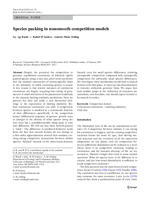
 Rafael D'Andrea