International Journal of Marine Engineering Innovation and Research, Vol. 1(4), Sept. 2017. 317-329 (pISSN: 2541-5972, eISSN: 2548-1479) 317 Risk Based Inspection of Gas-Cooling Heat Exchanger Dwi Priyanta1, Nurhadi Siswantoro2, Alfa Muhammad Megawan3 Abstract PHE – ONWJ platform personnel found 93 leaking tubes locations in the fin fan coolers/ gas-cooling heat exchanger. After analysis had been performed, the crack in the tube strongly indicate that stress corrosion cracking was occurred by chloride. Chloride stress corrosion cracking (CLSCC) is the cracking occurred by the combined influence of tensile stress and a corrosive environment. CLSCC is the one of the most common reasons why austenitic stainless steel pipework or tube and vessels deteriorate in the chemical processing, petrochemical and maritime industries. In this research purpose to determine the appropriate inspection planning for two main items (tubes and header box) in the gascooling heat exchanger using risk based inspection (RBI) method. The result, inspection of the tubes must be performed on July 6, 2024 and for the header box inspection must be performed on July 6, 2025. In the end, RBI method can be applicated to gas-cooling heat exchanger. Because, risk on the tubes can be reduced from 4.537 m2/year to 0.453 m2/year. And inspection planning for header box can be reduced from 4.528 m2/year to 0.563 m2/year. Keywords chloride stress corrosion cracking, inspection plan, RBI. I. 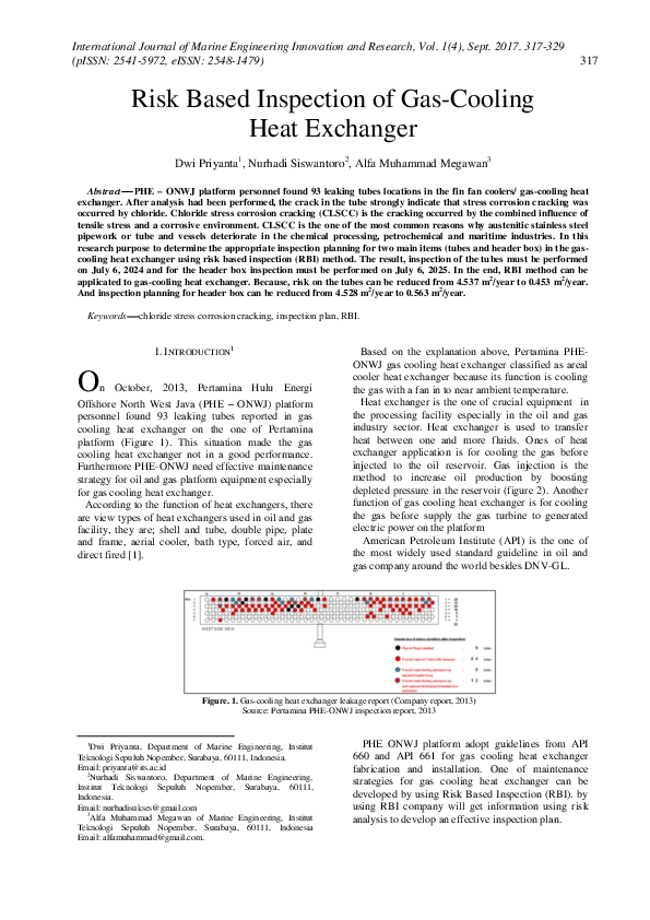INTRODUCTION1 O n October, 2013, Pertamina Hulu Energi Offshore North West Java (PHE – ONWJ) platform personnel found 93 leaking tubes reported in gas cooling heat exchanger on the one of Pertamina platform (Figure 1). This situation made the gas cooling heat exchanger not in a good performance. Furthermore PHE-ONWJ need effective maintenance strategy for oil and gas platform equipment especially for gas cooling heat exchanger. According to the function of heat exchangers, there are view types of heat exchangers used in oil and gas facility, they are; shell and tube, double pipe, plate and frame, aerial cooler, bath type, forced air, and direct fired [1]. Based on the explanation above, Pertamina PHEONWJ gas cooling heat exchanger classified as areal cooler heat exchanger because its function is cooling the gas with a fan in to near ambient temperature. Heat exchanger is the one of crucial equipment in the processing facility especially in the oil and gas industry sector. Heat exchanger is used to transfer heat between one and more fluids. Ones of heat exchanger application is for cooling the gas before injected to the oil reservoir. Gas injection is the method to increase oil production by boosting depleted pressure in the reservoir (figure 2). Another function of gas cooling heat exchanger is for cooling the gas before supply the gas turbine to generated electric power on the platform American Petroleum Institute (API) is the one of the most widely used standard guideline in oil and gas company around the world besides DNV-GL. Figure. 1. Gas-cooling heat exchanger leakage report (Company report, 2013) Source: Pertamina PHE-ONWJ inspection report, 2013 1 Dwi Priyanta, Department of Marine Engineering, Institut Teknologi Sepuluh Nopember, Surabaya, 60111, Indonesia. Email: priyanta@its.ac.id 2 Nurhadi Siswantoro, Department of Marine Engineering, Institut Teknologi Sepuluh Nopember, Surabaya, 60111, Indonesia. Email: nurhadisukses@gmail.com 3 Alfa Muhammad Megawan of Marine Engineering, Institut Teknologi Sepuluh Nopember, Surabaya, 60111, Indonesia Email: alfamuhammad@gmail.com. PHE ONWJ platform adopt guidelines from API 660 and API 661 for gas cooling heat exchanger fabrication and installation. One of maintenance strategies for gas cooling heat exchanger can be developed by using Risk Based Inspection (RBI). by using RBI company will get information using risk analysis to develop an effective inspection plan. International Journal of Marine Engineering Innovation and Research, Vol. 1(4), Sept. 2017. 317-329 (pISSN: 2541-5972, eISSN: 2548-1479) Identification of company equipment is the beginning of the systematic process in the inspection planning. Probability of failure and consequence of failure are the basic formula to calculate the RBI and must be evaluated by considering all damage mechanism directly effect to the equipment or the system. However, failure scenarios according to the actual damage mechanism should be develop and considered. 318 RBI methodology produces optimal inspection planning for the asset and make the priority from the lower risk to the higher risk. In other word inspection planning in RBI focused to identification what to inspect, how to inspect, where to inspect and how often to inspect. Inspection planning used to control degradation of the asset and the company will get considerable impact in the system operation and the appropriate economic consequences [2-18]. Figure. 2. optimization oil production by gas injection method II. METHOD The information of inspection planning in risk based inspection based on the risk analysis of the equipment. The purpose of the risk analysis is to identify the potential degradation mechanisms and threats to the integrity of the equipment and to assess the consequences and risk of failure [3]. A. Risk Risk is defined as the combination probability of asset failure and consequence if the failure happened. Risk can be expressed numerically with formula (1) as shown below. Risk = Probability x Consequence (1) Probability of Failure The probability of failure may be determined based on one, or a combination of the following methods: - Structural reliability models In this method, a limit state is defined based on a structural model that includes all relevant damage mechanisms, and uncertainties in the independent variables of this models are defined in terms of statistical distributions. The resulting model is solved directly for the probability of failure. - Statistical models based on generic data In this method, generic data is obtained for the component and damage mechanism under evaluation and a statistical model is used to evaluate the probability of failure. - Expert judgment In this method, expert solicitation is used to evaluate the component and damage mechanism, a probability of failure can typically only be assigned on a relative basis using this method. In API RBI, a combination of the above is used to evaluate the probability of failure in terms of a generic failure frequency and damage factor. The probability of failure calculation is obtained from the equation (2). Pof (t) = gff x Df (t) x FMS (2) Where: gff = generic failure frequency Df (t) = damage factor FMS = management system factor B. Generic Failure Frequency (gff) The generic failure frequency can be determined by asset failure of common industries. The generic failure frequency is expected to the previous failure International Journal of Marine Engineering Innovation and Research, Vol. 1(4), Sept. 2017. 317-329 (pISSN: 2541-5972, eISSN: 2548-1479) frequency to any specific damage happening from exposure to the operating environment. There are four different damage hole sizes model the release scenarios covering a full range of events they are small, medium, large, and rupture. If the data of the asset is complete, actual probabilities of the failure could be calculated with actual observed failures. Even if a failure has not occurred in a component, the true probability of failure is likely to be greater than zero because the component may not have operated long enough to experience a failure. As a first step in estimating this non-zero probability, it is necessary to examine a larger set of data of similar components to find enough failures such that a reasonable estimate of a true probability of failure can be made. This generic component set of data is used to produce a generic failure frequency for the component. The generic failure frequency of a component type is estimated using records from all plants within a company or from various plants within an industry, from literature sources, and commercial reliability data bases. Therefore, these generic values typically represent an industry in 319 general and do not reflect the true failure frequencies for a specific component subject to a specific damage mechanism. The generic failure frequency is intended to be the failure frequency representative of failures due to degradation from relatively benign service prior to accounting for any specific operating environment, and are provided for several discrete hole sizes for various types of processing equipment (i.e. process vessels, drums, towers, piping systems, tankage, etc.). A recommended list of generic failure frequencies is provided in Table 1. The generic failure frequencies are assumed to follow a log-normal distribution, with error rates ranging from 3% to 10%. Median values are given in Table 1. The data presented in the Table 1 is based on the best available sources and the experience of the API RBI Sponsor Group. The overall generic failure frequency for each component type was divided across the relevant hole sizes, i.e. the sum of the generic failure frequency for each hole size is equal to the total generic failure frequency for the component. TABLE 1 SUGGESTED COMPONENT GENERIC FAILURE FREQUENCIES (GFF) gff as a Function of Hole Size (failures/yr) gff(total) Equipment type Component type Pipe PIPE-1 Vessel/ FinFan FINFAN Small Medium Large 2.80E-05 0 0 8.00E-06 2.00E-05 2.00E-06 C. Management System Factor Management system factor used to measure how good the facility management system that may arise due to an accident and labor force of the plant is trained to handle the asset. This evaluation consists of a series of interviews with plant management, operations, inspection, maintenance, engineering, training, and safety personnel. The management systems evaluation procedure developed for API RBI covers all areas of a plant’s PSM system that impact directly or indirectly on the mechanical integrity of process equipment. The management systems evaluation is based in large part on the requirements contained in API Recommended Practices and Inspection Codes. It also includes other proven techniques in effective safety management. A listing of the subjects covered in the management systems evaluation and the weight given to each subject is presented in Table 2. The management systems evaluation covers a wide range of topics and, as a result, requires input from several different disciplines within the facility to Rupture (failures/yr) 2.60E-06 3.06E-05 6.00E-07 3.06E-05 answer all questions. Ideally, representatives from the following plant functions should be interviewed: a) Plant Management b) Operations c) Maintenance d) Safety e) Inspection f) Training g) Engineering The scale recommended for converting a management systems evaluation score to a management systems factor is based on the assumption that the “average” plant would score 50% (500 out of a possible score of 1000) on the management systems evaluation, and that a 100% score would equate to a one order-of magnitude reduction in total unit risk. Based on this ranking, equation (3) and equation (4) may be used to , for any compute a management systems factor, management systems evaluation score. International Journal of Marine Engineering Innovation and Research, Vol. 1(4), Sept. 2017. 317-329 (pISSN: 2541-5972, eISSN: 2548-1479) 320 TABLE 2 MANAGEMENT SYSTEMS EVALUATION Table Title Points 2.A.1 Leadership and Administration 6 70 2.A.2 Process Safety Information 10 80 2.A.3 Process Hazard Analysis 9 100 2.A.4 2.A.5 Management of Change Operating Procedures 6 7 80 80 2.A.6 Safe Work Practices 7 85 2.A.7 Training 8 100 2.A.8 Mechanical Integrity 20 120 2.A.9 Pre-Startup Safety Review 5 60 2.A.10 Emergency Response 6 65 2.A.11 Incident Investigation 9 75 2.A.12 2.A.13 Total Contractors Audits 5 4 102 45 40 1000 *Note that the management score must first be converted to a percentage (between 0 and 100) as follows: (3) (4) D. Thinning Damage Factor The calculation procedures of thinning damage factor are: a) Determine the number of inspections, and the corresponding inspection effectiveness category for all past inspections. Combine the inspections to the highest effectiveness performed. b) Determine the time in-service (age) since the last inspection thickness reading (trd). c) Determine the corrosion rate for the base metal (Cr,bm) based on the material of construction and process environment, where the component has cladding, a corrosion rate (Cr,cm) must also be obtained for the cladding. d) Determine the minimum required wall thickness per the original construction code or using ( API 579. If the component is a tank bottom, then = 0.1 in) if the in accordance with API 653 ( tank does not have a release prevention barrier and ( = 0.05 in) if the tank has a release prevention barrier. e) For clad components, calculate the time or age from the last inspection required to corrode away , using equation (5). the clad material, = max [( Questions = N/A (5) f) Determine the parameter using Equation below, based on the age and from step b, from step c, from step d and the age required to corrode away the cladding, , if applicable from step e. For components without cladding, and for components where the cladding is corroded away at the time of the last inspection = 0.0), use Equation (6). (i.e. (6) g) Determine the damage factor for thinning, using Equation (2.13). , (7) E. Stress Corrosion Cracking Damage Factor The calculation procedures of chloride stress corrosion cracking (CL-SCC) damage factor are: a) Determine the number of inspections, and the corresponding inspection effectiveness category for all past inspections. Combine the inspections to the highest effectiveness performed. b) Determine the time in-service (age) since the last Level A, B, C or D inspection was performed. c) Determine the susceptibility for cracking using Table 3 based on the operating temperature and concentration of the chloride ions. Note that a HIGH susceptibility should be used if cracking is known to be present. International Journal of Marine Engineering Innovation and Research, Vol. 1(4), Sept. 2017. 317-329 (pISSN: 2541-5972, eISSN: 2548-1479) 321 TABLE 3 SUSCEPTIBILITY TO CRACKING – CLSCC pH ≤ 10 Susceptibility to Cracking as a Function of Chloride ion (ppm) Temperature (°C) 1-10 11-100 101-1000 >1000 38 – 66 Low Medium Medium High >66 – 93 Medium Medium High High >93 – 149 Medium High High High pH > 10 Susceptibility to Cracking as a Function of Chloride ion (ppm) Temperature (°C) 1-10 11-100 101-1000 >1000 < 93 Low Low Low Low 93 -149 Low Low Low Medium TABLE 4 DETERMINATION OF SEVERITY INDEX – CLSCC Susceptibility Severity Index – SVI High 5000 Medium 500 Low 50 None 1 d) Based on the susceptibility in step c, and from table (4). determine the severity index, e) Determine the base damage factor for CLSCC, using table (5) based on the number of, and the highest inspection effectiveness determined in step a, and the severity index, , from step d. inspection using the age from step b and equation below. In this equation, it is assumed that the probability for cracking will increase with time since the last inspection as a result of increased exposure to upset conditions and other non-normal conditions. f) Calculate the escalation in the damage factor based on the time in-service since the last = (age)1.1 (8) TABLE 5 SCC DAMAGE FACTORS – ALL SCC MECHANISMS SVI E Inspection Effectiveness 2 Inspections 1 Inspection 3 Inspections D C B A D C B A D C B A 1 1 1 1 1 1 1 1 1 1 1 1 1 1 10 10 8 3 1 1 6 2 1 1 4 1 1 1 50 50 40 17 5 3 30 10 2 1 20 5 1 1 100 100 80 33 10 5 60 20 4 1 40 10 2 1 500 500 400 170 50 25 300 100 20 5 200 50 8 1 1000 1000 800 330 100 50 600 200 40 10 400 100 16 2 5000 5000 4000 1670 500 250 3000 1000 250 50 2000 500 80 10 F. Consequence Analysis The calculations of consequence procedures are: a) Select a representative fluid group from Table 6. International Journal of Marine Engineering Innovation and Research, Vol. 1(4), Sept. 2017. 317-329 (pISSN: 2541-5972, eISSN: 2548-1479) b) Determine the stored fluid properties using equation (9) and Table 7 (MW: Molecular weight; k: ideal gas specific ratio, AIT: Auto Ignition Temperature). 8 and the phase of the fluid stored in the equipment as determined in step b. d) Based on the component type and Table 9, determine the release hole size diameters (dn). (9) e) Determine the steady state phase of the fluid Determine the generic failure frequency (gffn), and the total generic failure frequency from this table or from equation (10). after release to the atmosphere, using Table (10) TABLE 6 LIST OF REPRESENTATIVE FLUIDS AVAILABLE FOR LEVEL 1 ANALYSIS Representative Fluid Fluid TYPE C₁ -C₂ TYPE 0 methane, ethane, ethylene, LNG, fuel gas C₃ -C₄ TYPE 0 propane, butane, isobutane, LPG C₅ TYPE 0 Pentane C₆ -C₈ TYPE 0 gasoline, naptha, light stright run, heptane C₉ -C₁ ₂ TYPE 0 diesel, kerosene TYPE 0 jet fuel, kerosene, atmospheric gas oil C₁ ₇ -C₂ ₅ TYPE 0 gas oil, typical crude C₁ ₃ -C₁ ₆ Examples of Applicable Materials TABLE 7 PROPERTIES OF THE REPRESENTATIVE FLUIDS USED IN LEVEL 1 ANALYSIS Liquid Density (kg/m³) NBP (°C) Ambient State Ideal Gas Specific Heat Eq. Ideal Gas Constant A Ideal Gas Constant B Ideal Gas Constant C Ideal Gas Constant D Ideal Gas Constant E C₁ -C₂ 23 250.512 -125 Gas Note 1 12.3 1.15E-01 -2.87E-05 -1.30E-09 N/A 558 C₃ -C₄ 51 538.379 -21 Gas Note 1 2.632 0.3188 -1.35E+04 1.47E-08 N/A 369 C₅ 72 625.199 36 Liquid Note 1 -3.626 0.4873 -2.60E-04 5.30E-08 N/A 284 100 684.018 99 Liquid Note 1 -5.146 6.76E-01 -3.65E-04 7.66E-08 N/A 223 C₆ -C₈ C₉ 149 734.012 C₁ ₂ C₁ ₃ 205 764.527 C₁ ₆ C₁ ₇ 280 775.019 C₂ ₅ C₂ ₅ ₊ 422 900.026 Auto-Ignition Temp. (°C) MW Cp Fluid c) 322 184 Liquid Note 1 -8.5 1.01E+00 -5.56E-04 1.18E-07 N/A 208 261 Liquid Note 1 -11.7 1.39E+00 -7.72E-04 1.67E-07 N/A 202 344 Liquid Note 1 -22.4 1.94E+00 -1.12E-03 -2.53E-07 N/A 202 527 Liquid Note 1 -22.4 1.94E+00 -1.12E-03 -2.53E-07 N/A 202 International Journal of Marine Engineering Innovation and Research, Vol. 1(4), Sept. 2017. 317-329 (pISSN: 2541-5972, eISSN: 2548-1479) 323 TABLE 8 CONSEQUENCE ANALYSIS GUIDELINES FOR DETERMINING THE PHASE OF A FLUID Phase of Fluid at Normal Operating (Storage) Conditions Phase of Fluid at Ambient (after release) Conditions API RBI Determination of Final Phase for Consequence Calculation Gas Gas model as gas Gas Liquid model as gas Liquid Gas model as gas unless the fluid boiling point at ambient conditions is greater than 80°F, then model as a liquid Liquid Liquid model as liquid TABLE 9 RELEASE HOLE SIZES AND AREA USED Release Hole Number Release Hole Size Range of Hole Diameters (mm) Release Hole Diameter, dn (mm) 1 Small 0 – 6.4 D1 = 6.4 2 Medium >6.4 – 51 D2 = 25 3 Large >51 – 152 D3 = 102 4 Rupture >152 D4 = min[D, 406] f) Select the appropriate release rate equation as described above using the stored fluid phase g) For each release hole size, compute the release hole size area (An) using equation (11). = (11) h) For each release hole size, calculate the release rate (Wn) with equation (12) for each release area (An) = x x i) Group components and equipment items into inventory groups using Table 10. j) Calculate the fluid mass (masscomp) in the component being evaluated. k) Calculate the fluid mass in each of the other components that are included in the inventory group (masscomp,i). l) Calculate the fluid mass in the inventory group (massinv) using Equation (13). (13) x (12) TABLE 10 ASSUMPTION WHEN CALCULATING LIQUID INVENTORIES WITHIN EQUIPMENT Equipment Description Component Type Knock-out Pots and Dryers Compressors Heat Exchangers Fin Fan Air Coolers KODRUM COMPC COMPR COMPR HEXSS HEXTS FINFAN Examples Default Liquid Volume Percent Compressor Knock-outs, Fuel Gas KO Drums, Flare Drums, Air Dryers. 10% liquid Much less liquid inventory expected in knock-out drums Centrifugal and Reciprocating Compressors Negligible, 0% Shell and Tube Heat Exchangers Total Condensers, Partial Condensers, Vapor Coolers and Liquid Coolers 50% shell-side, 25% tube-side 25% liquid Filters FILTER 100% full Piping PIPE-xx 100% full, calculated for Level 2 Analysis International Journal of Marine Engineering Innovation and Research, Vol. 1(4), Sept. 2017. 317-329 (pISSN: 2541-5972, eISSN: 2548-1479) m) Calculate the flow rate from a 203 mm [8 in] diameter hole (Wmax8) using equations above, as applicable, with An = A8 = 32,450 mm2 [50.3 in2]. This is the maximum flow rate that can be added to the equipment fluid mass from the surrounding equipment in the inventory group. n) For each release hole size, calculate the added fluid mass (massadd,n) with equation (14) resulting from three minutes of flow from the inventory group using equation below where W n is the leakage rate for the release hole size being evaluated and Wmax8 is from last step. massadd,n = 180 . min [Wn , Wmax8] (14) o) For each release hole size, calculate the available mass for release using equation (15). Massavail,n = min[{masscomp + massadd,n}, massinv] (15) p) For each release hole size, calculate the time required to release 4,536 kgs [10,000 lbs] of fluid. (16) q) For each release hole size, determine if the release type is instantaneous or continuous using the following criteria. - If the release hole size is 6.35 mm [0.25 inches] or less, then the release type is continuous. - If 180 tn ≤ sec or the release mass is greater than 4,536 kgs [10,000 lbs], then the release is instantaneous; otherwise, the release is continuous r) Determine the detection and isolation systems present in the unit. s) Using Table 11 select the appropriate classification (A, B, C) for the detection system. TABLE 11 DETECTION AND ISOLATION SYSTEM RATING GUIDE Type of Detection System Detection Classification Instrumentation designed specifically to detect material losses by changes in operating conditions (i.e., loss of pressure or flow) in the system A Suitably located detectors to determine when the material is present outside the pressure-containing envelope B Visual detection, cameras, or detectors with marginal coverage C Type of Isolation System Isolation Classification Isolation or shutdown systems activated directly from process instrumentation or detectors, with no operator intervention A Isolation or shutdown systems activated by operators in the control room or other suitable locations remote from the leak B Isolation dependent on manually-operated valves C TABLE 12 ADJUSTMENTS TO RELEASE BASED ON DETECTION AND ISOLATION SYSTEMS System Classifications Release Magnitude Adjustment Reduction Factor, factdi A Reduce release rate or mass by 25% 0.25 A B Reduce release rate or mass by 20% 0.20 A or B C Reduce release rate or mass by 10% 0.10 B B Reduce release rate or mass by 15% 0.15 C C No adjustment to release rate to mass 0.00 Detection Isolation A 324 International Journal of Marine Engineering Innovation and Research, Vol. 1(4), Sept. 2017. 317-329 (pISSN: 2541-5972, eISSN: 2548-1479) 325 TABLE 13 LEAK DURATIONS BASED ON DETECTION AND ISOLATION SYSTEMS Detecting System Rating Isolation System Rating Maximum Leak Duration, ldmax 20 minutes for 6.4 mm leaks A A 10 minutes for 25 mm leaks 5 minutes for 102 mm leaks 30 minutes for 6.4 mm leaks A B 20 minutes for 25 mm leaks 10 minutes for 102 mm leaks 40 minutes for 6.4 mm leaks A C 30 minutes for 25 mm leaks 20 minutes for 102 mm leaks 40 minutes for 6.4 mm leaks B A or B 30 minutes for 25 mm leaks 20 minutes for 102 mm leaks t) Using Table 11 select the appropriate classification (A, B, C) for the isolation system. u) Using Table 12 and the classifications determined in step s & t, determine the release reduction factor, factdi. v) Using Table 13 and the classifications determined in step s & t, determine the total leak durations for each of the selected release hole sizes, ldmax,n. w) For each release hole size, calculate the adjusted release rate (raten) using equation (17) where the theoretical release rate (Wn). raten = Wn(1-factdi) (17) x) For each release hole size, calculate the leak duration (ldn) of the release using Equation 4.13, based on the available mass (massavail,n), and the adjusted release rate (raten) from step. Note that the leak duration cannot exceed the maximum duration (Idmax,n) determined in step w. (18) y) For each release hole size, calculate the release mass (massn), using equation (19) based on the release rate (raten), the leak duration (ldn), and the available mass (massavail,n). massn = min [{raten . ldn} , massavail,n] (19) Select the consequence area mitigation reduction factor (factmit) from Table 14. aa) b For each release hole size, calculate the energy efficiency correction factor, (eneffn) using equation below. z) – 15 (20) bb) Determine the fluid type, either TYPE 0 or TYPE 1 from Table 6. cc) For each release hole size, compute the component damage consequence areas for Autoignition Not Likely, Continuous Release (AINL-CONT) - - Determine the appropriate constants a ( and b ( from the Table 15 will be needed to assure selection of the correct constants. If the release is a gas or vapor and the fluid type is TYPE 0, then use equation (21) for the consequence area and for the release rate. = x (21) International Journal of Marine Engineering Innovation and Research, Vol. 1(4), Sept. 2017. 317-329 (pISSN: 2541-5972, eISSN: 2548-1479) 326 TABLE 14 ADJUSTMENTS TO FLAMMABLE CONSEQUENCES FOR MITIGATION SYSTEMS Mitigation System Consequence Area Adjustment Consequence Area Reduction Factor (factmit) Inventory blowdown, coupled with isolation system classification B or higher Reduce consequence area by 25% 0.25 Fire water deluge system and monitors Reduce consequence area by 20% 0.20 Fire water monitors only Reduce consequence area by 5% 0.05 Foam spray system Reduce consequence area by 15% 0.15 TABLE 15 COMPONENT DAMAGE FLAMMABLE CONSEQUENCE EQUATION CONSTANTS Continuous Releases Constants Auto-Ignition Not Likely Auto-Ignition Likely (CAINL) (CAIL) Fluid Gas Liquid a b b C₁ -C₂ 8.669 C₃ -C₄ 10.13 0.98 55.13 0.95 1.00 64.23 1.00 C₅ 5.115 0.99 100.6 0.89 62.41 1.00 C₆ -C₈ 5.846 0.98 34.17 0.89 63.98 C₉ -C₁ ₂ 2.419 0.98 24.6 0.90 76.98 12.11 C₁ ₇ -C₂ ₅ C₂ ₅ ₊ B Liquid A C₁ ₃ -C₁ ₆ a Gas a B 1.00 103.4 0.95 0.95 110.3 0.95 0.90 196.7 0.92 3.785 0.90 165.5 0.92 2.098 0.91 103.0 0.90 Instantaneous Releases Constants Auto-Ignition Not Likely Auto-Ignition Likely (IAINL) (IAIL) Fluid Gas Liquid a b A b 6.469 0.67 163.7 0.62 C₃ -C₄ 4.590 0.72 79.94 0.63 C₅ 2.214 0.72 0.271 0.85 41.38 0.61 C₆ -C₈ 2.188 0.66 0.749 0.78 41.49 C₉ -C₁ ₂ 1.111 0.66 0.559 0.76 42.28 0.086 0.88 0.021 0.006 C₁ ₇ -C₂ ₅ C₂ ₅ ₊ dd) For each release hole size, compute the component damage consequence areas for Autoignition Likely, Continuous Release (AILCONT), ( B Liquid C₁ -C₂ C₁ ₃ -C₁ ₆ a Gas a B 0.61 8.180 0.55 0.61 0.848 0.53 1.714 0.88 0.91 1.068 0.91 0.99 0.284 0.99 - Determine the appropriate constants, a ( and b ( The release phase will be needed to assure selection of the correct constants. International Journal of Marine Engineering Innovation and Research, Vol. 1(4), Sept. 2017. 317-329 (pISSN: 2541-5972, eISSN: 2548-1479) ignition Likely, Continuous Release (AILCONT) ( - If the release type is gas or vapor, Type 0 or Type 1, then use equation (21) to compute the consequence area and compute the effective release rate. = - x (22) - ee) For each release hole size, compute the component damage consequence areas for Autoignition Not Likely, Instantaneous Release (AINL-INST) - Determine the appropriate constants a ( and b ( . The release phase will be needed to assure selection of the correct constants. - If the release is a gas or vapor and the fluid type is TYPE 0, or the fluid type is TYPE 1, then use equation (23) for the consequence area and the effective release rate. = x x (26) For each release hole size, compute the personnel injury consequence areas for Autoignition Not Likely, Instantaneous Release (AINL-INST) ( - - ff) For each release hole size, compute the component damage consequence areas for Autoignition Likely, Instantaneous Release (AIL-INST) ( x (24) gg) For each release hole size, compute the personnel injury consequence areas for Autoignition Not Likely, Continuous Release (AINLCONT) ( - Determine the appropriate constants a and b . The ( release phase will be needed to assure selection of the correct constants. - Compute the consequence area using Equation (25) where is from step cc. = x (25) Determine the appropriate constants a ) and b ( . The release phase will be needed to assure selection of the correct constants. Compute the consequence area using equation (27) where = ii) For each release hole size, compute the personnel injury consequence areas for Autoignition Likely, Instantaneous Release (AILINST) ( - Determine the appropriate constants a ) and b ( . The release ( phase will be needed to assure selection of the correct constants. Compute the consequence area using equation (28) where . = x (28) jj) For each release hole size, calculate the instantaneous/continuous blending factor ( . - For Continuous Releases – To smooth out the results for releases that are near the continuous to instantaneous transition point (4,536 kgs [10,000 lbs] in 3 minutes, or a release rate of 25.2 kg/s [55.6 lb/s]), then the blending factor use equation (29). = min hh) For each release hole size, compute the personnel injury consequence areas for Auto- x (27) = Determine the appropriate constants a ) and b . The release ( phase will be needed to assure selection of the correct constants. Compute the consequence area using equation (26) where = (23) - Determine the appropriate constants a ( and b ( . The release phase will be needed to assure selection of the correct constants. - If the release type is gas or vapor, Type 0 or Type 1, then use equation (24) to compute the consequence area and to compute the effective release rate. 327 (29) - For Instantaneous Releases – Blending is not required. Since the definition of an International Journal of Marine Engineering Innovation and Research, Vol. 1(4), Sept. 2017. 317-329 (pISSN: 2541-5972, eISSN: 2548-1479) instantaneous release is one with a adjusted release rate (raten) greater than 25.2 kg/s [55.6 lb/s] (4536 kg [10,000 lbs] in 3 minutes), then the blending factor use equation (30). = 1.0 kk) 328 mm) Compute the AIT blended consequence areas for the component using equations (36) and (37). The resulting consequence areas are the component damage and personnel injury flammable consequence areas. (30) , Calculate the AIT blending factor using some equations, as applicable. Since Ts (450.15 kelvin) + C₆ (56) < AIT (831.150) then the equation (313) (36) (31) (37) ll) Compute the continuous/instantaneous blended consequence areas for the component using equations (32) – (35). (32) nn) Determine the final consequence areas (probability weighted on release hole size) for component damage and personnel injury using equations below. = (38) = (39) (33) (34) III. RESULT (35) The result of calculation shown in the Table 16 and 17. TABLE 16 CALCULATION RESULTS SUMMARIES FOR TUBE Damage factor at RBI date 3790.5977 Damage factor at plan date 8716.0138 Total generic failure frequency 0.0000306 Total factor management system 50% Probability of failure (RBI date) 0.083562 Probability of failure (Plan date) 0.197204 Total consequence area for equipment damage 14.07017389 m2 Total consequence area for personnel injury 34.02010644 m2 Risk at RBI date 1.973035017 m2/year Risk at Plan Date 4.536751674 m2/year Risk target Next inspection date Risk Area with Inspection 3.71612 m2/year 12/20/2019 0.29248 m2/year International Journal of Marine Engineering Innovation and Research, Vol. 1(4), Sept. 2017. 317-329 (pISSN: 2541-5972, eISSN: 2548-1479) 329 TABLE 17 CALCULATION RESULTS SUMMARIES FOR HEADER BOX Damage factor at RBI date 7154.9457 Damage factor at plan date 30448.3875 Total generic failure frequency 0.0000306 Total factor management system 50% Probability of failure (RBI date) 0.109471 Probability of failure (Plan date) 0.111739 Total consequence area for equipment damage 4.020049682 m2 Total consequence area for personnel injury 9.720030412 m2 Risk at RBI date 1.064058236 m2/year Risk at Plan Date 4.528176567 m2/year Risk target Next inspection date Risk Area with Inspection IV. CONCLUSION According to the analysis of the research study, then some conclusion could be taken as explain below: 1. There are two damage factors obtained for the tube and header box. They are; thinning damage factor and CL-SCC damage factor and the result of the damage factor for the header box is 7154.95 at RBI date and 30448.4 at plan date. For the tube, the damage factor is 2720.62 at RBI date and 4158.99 at the plan date. 2. The risk area value for the tubes in the new inspection plan is 0.29248 m2/year and for the header box the new inspection plan is 0.56251 m2/year. 3. The inspection planning for the tubes could be generated on July 6, 2024 and inspection planning for the header box could be generated on July 6, 2025. 4. Remaining life for the asset is 8.696 years. REFERENCES [1] K. Arnold and M. Stewart, Surface Production Operation Volume 2, Houston, Texas: Gulf Publishing Company, 1989. [2] M. H. Faber, "Risk Based Inspection Maintenance Planning," Risk Based Inspection Maintenance Planning, p. 3, 2001. [3] M. B. W. K. J B Wintle and S. S. G J Amphlett, Best practice for risk based inspection, Norwich: Crown, 2001. [4] M. S. Ken Arnold, Surface Production Volume 2, Houston: Gulf Publishing Company, 1999. 3.71612 m2/year 07/06/2025 0.56251 m2/year [5] American Petroleum Institute, Air-Cooled heat Exchangers for General Refinery System, 6th ed., Washington: API Publishing Service, 2006. [6] BPPT, "Analisa Kerusakan Fin Tube Air Cooler PHE," Balai Besar Teknologi Kekuatan Struktur (B2TKS) - BPPT, Serpong, 2013. [7] National Physical Laboratory, "Guides to Good Practice in Corrosion Control," Stress Corrosion Cracking, p. 4, 2000. [8] American Petroleum Institute, Procedures for Standards Development, 4th ed., Washington: American Petroleum Institute, 2011. [9] American Petroleum institute, Risk Based Inspection Technology, Washington, D.C.: API Publishing Service, 2008. [10] American Petroleum Institute, Shell-and-tube Heat Exchangers, 8th ed., Washington: American Petroleum Institute, 2007. [11] PT. LAPI ITB, "Tube to Tube Sheet Expansion Review and Thermal Stress Design Review For FFC Hal-200 Leaking Tube Root Cause Analysis," PT. LAPI ITB, Bandung, 2013. [12] Ravi K. Sharma a, "Automation of emergency response for petroleum oil storage terminals," Safety Science, pp. 1-12, 2015. [13] Kaley, "Documenting and Demonstrating the Thinning," API RP 581 Risk-Based Inspection Methodology, p. 3, November 2014. [14] Prastowo H, Fitri S P, Gruning S. “Design of High Rate Blender Hydraulic Power Pack Unit on Stimulation Vessel – Study Case Stim Star Borneo for Offshore Operations at Delta Mahakam area – East Borneo”. International Journal of Marine Engineering Innovation and Research., vol. 1, no. 2, Mar. 2017.