AGRICULTURAL
SYSTEMS
Agricultural Systems 92 (2007) 266–294
www.elsevier.com/locate/agsy
Economics of alternative simulated manual
asparagus harvesting strategies
Tiziano Cembali *, Raymond J. Folwell, Ray G. Huffaker,
Jill J. McCluskey, Phil R. Wandschneider
School of Economic Sciences, Washington State University, P.O. Box 646210,
Pullman, WA 99164-6210, United States
Received 30 November 2004; received in revised form 23 March 2006; accepted 30 March 2006
Abstract
Asparagus is harvested daily during the production season. The adoption of harvesting
strategies less or more frequent than the traditional 24-h strategy has not occurred because
of problems in hiring manual labor. A model that predicts daily harvest and the impact of different harvesting strategies was developed. This paper presents a bioeconomic model, capable
of predicting daily asparagus harvests, composed by different mathematical functions: emergence, density dynamics, spear growth, diameter, weight, carbohydrates reserve dynamics,
and profit. The bioeconomic model was used to simulate yield, number of harvests, profit,
and the total cost of harvest for every year in the period 1989–2004. A simulation with the
minimum wage harvesting constraint was developed and is labeled as the constrained model.
The model was evaluated using data from different locations for four consecutive years in
Washington State (USA) asparagus fields. The impact of the minimum wage requirements
was estimated in terms of yield and profit for both processed and fresh asparagus. The traditional harvest interval of 24 h was compared to a more frequent (12 h) and a less frequent
(48 h) interval. Manual harvest with the interval of 12 h showed the best results in terms of
yields and profits for both processed and fresh asparagus. Gains in profits with the actual production conditions in Washington State were US$183.88/ha and US$210.60/ha for processed
and fresh product, respectively. The 48-h strategy resulted in decreased yields and profits.
2006 Elsevier Ltd. All rights reserved.
*
Corresponding author. Tel.: +1 509 335 5556; fax: +1 509 335 1173.
E-mail address: tizianocembali@yahoo.com (T. Cembali).
0308-521X/$ - see front matter 2006 Elsevier Ltd. All rights reserved.
doi:10.1016/j.agsy.2006.03.009
T. Cembali et al. / Agricultural Systems 92 (2007) 266–294
267
Keywords: Asparagus; Harvest; Bioeconomic model; Mathematical model; Simulation
1. Introduction
Asparagus is generally harvested daily during the production season. The daily
harvesting decision depends upon whether or not sufficient spear growth has
occurred in the asparagus bed to justify the harvesting expense since the last harvest.
The actual harvesting usually occurs only once each day starting in the early morning and ending in the early afternoon. The yield maximizing harvesting strategy
would be to cut a spear as it reaches the desirable length, so multiple daily harvests
would be needed to maximize yields. This is because the energy used by the plant
(crown) can be directed toward new spears rather than adding length to spears that
are already at the required length for harvest and marketing.
By law in the State of Washington (USA) as well as in the rest of the United
States, manual labor is paid at least the minimum wage. Considering that asparagus
growers pay a per unit amount to the manual labor to harvest asparagus, the harvesting becomes reality only when the revenue (quantity times the price per unit
received) is at least equal to the minimum wage pay for the workers. The grower
must make some monetary augmentations to guarantee the minimum wages if pay
received for harvesting by manual labor does not meet this condition. This represents
a constraint on the competitiveness of the Washington (USA) asparagus industry
because the minimum wage is the highest in USA (US$7.16/h for 2003) (DOL, 2004).
Daily harvests remain the common practice. Increasing the number of harvests
per day would mean multiple cuttings per day. This has not been done because of
the difficulty in recruiting manual labor willing to harvest in the afternoon when temperature are generally high. No research has been conducted to show the potential
production using such a harvesting strategy.
The adoption of a strategy with less frequent than daily harvests has not been considered profitable because an asparagus grower is paid on a given acceptable length
and any additional length to the spear is trimmed. By not harvesting daily, the quantity of asparagus trimmed (not payable) is greater because spears tend to be longer
than the required length. This creates a waste of carbohydrate (CHO) reserve that
could be used to produce a marketable or payable product.
The only research focused on harvest strategies was done by Lampert et al.
(1980). They addressed the issue of harvesting strategies using a simulation model.
Their approach considered the length of the harvesting season and the possibility
to skip a harvesting season every nth year. Stout et al. (1967) addressed this issue
of different frequency of harvest from an economic perspective, but they did not
relate the study to the biological response of plants with the different strategy. Neither of these research efforts addressed the issue of predicting daily harvests of
asparagus. Also, their modeling approach did not allow for evaluating different
harvesting strategies within a season considering the biological impact of such
strategies on the asparagus crown.
268
T. Cembali et al. / Agricultural Systems 92 (2007) 266–294
A bioeconomic growth simulation model for asparagus capable of predicting
daily harvest is a necessary tool to analyze alternative harvesting strategies. Due
to harvesting issues, asparagus field experiments can be extremely expensive. In addition, variability in weather conditions, pests, and weeds can affect the data of field
trials. A bioeconomic growth simulation model would represent the solution for preliminary screening of different harvesting strategies.
This paper represents the first attempt to address the issue of manual harvesting
using a bioeconomic model. The specific objectives of this paper are: (1) to present an
asparagus growth model capable to predict daily harvests; (2) to integrate the biological growth model with the economic decisions that the grower takes into account in
the harvesting decisions; and (3) to determine the impact on profits of different harvesting strategies involving frequencies of manual harvests.
This paper is organized into four sections: (1) model description; (2) methods; (3)
results and discussion; and (4) conclusions. In general, the model description section
is divided into: theoretical bioeconomic model, empirical bioeconomic model, biology and agronomy, and economics. The biology and agronomy subsection includes:
(1) emergence and density dynamics; (2) spear growth, diameter, and weight; (3)
CHO dynamics; and (4) production conditions.
2. Model description
2.1. The theoretical bioeconomic model
In the model it was assumed that the manager would select a harvesting intensity
that maximizes profit subject to the CHO constraint. In the model, harvesting is
stopped at the minimum CHO level in order to not negatively impact the production
in the following years. The number of asparagus spears harvested at time t (H(t))
represented the harvest intensity, that could be defined as the control variable in a
dynamic optimization framework. The CHO level and the total number of asparagus
in the field were the state variables of the model. In the theoretical model the payable
weight of a spear was a function of the plant’s reserve of CHO, in accordance to
Lampert et al. (1980). The harvesting costs were assumed decreasing as the number
of spears available for harvesting increased. This last assumption was made because
the higher the number of the spears available, the greater the efficiency of the manual
labor. The theoretical model can be written mathematically as:
max
T 1
X
½pH ðtÞPW ðCRðtÞÞ rðH ðtÞÞH ðtÞ1t
t¼0
s:t: CRðt þ 1Þ CRðtÞ ¼ H ðtÞW ðCRðtÞÞr
ð1Þ
N ðt þ 1Þ N ðtÞ ¼ EðtÞ H ðtÞ
where p is the price per unit of asparagus, H(t) is the number of asparagus spears harvested, PW(CR(t)) is the payable weight of asparagus expressed as an increasing function of the CHO reserve at time t, r(H(t)) is the harvesting cost and is identified as a
T. Cembali et al. / Agricultural Systems 92 (2007) 266–294
269
decreasing function of the number of asparagus spears harvested, 1t is the discount
1
term defined as ð1þdÞ
, where d is the daily discount rate, CR(t) is the CHO reserve at
time t, W(CR(t)) is the total weight of the spear at time t expressed as an increasing
function of the CHO reserve, r is the transformation coefficient of CHO into fresh
asparagus weight, N(t) is the number of spears of asparagus at time t, and E(t) is
the number of asparagus emerged at time t. Table 1 report the complete summary
of variables symbols, definitions, and units for all the variables used in the model.
Eq. (1) can solved using the Lagrange multiplier method. The Lagrangian expression of the problem, following Clark (1990, p. 235), is:
L¼
T 1
X
½pH ðtÞPW ðCRðtÞÞ rðH ðtÞÞHðtÞ1t þ kðtÞ½CRðt þ 1Þ CRðtÞ H ðtÞW ðCRðtÞÞr
þlðtÞ½N ðt þ 1Þ NðtÞ EðtÞ þ H ðtÞ
t¼0
ð2Þ
where k(t) and l(t) are shadow prices of a unit of CHO and a spear of asparagus,
respectively. The shadow price represents the amount that the objective function
would increase if the constraint were relaxed by one unit (e.g. an extra unit of
CHO would be available for the production). The initial and terminal values of
the state variable were given, CR(0) represented the initial CHO reserve (at time
0), and CR(T) represented the final CHO reserve (at time T). Therefore, harvest
was interrupted when CR(T) was less or equal to the minimum value of CHO
(CRmin).
The necessary conditions for optimality are:
oL
¼ ½pPW ðCRðtÞÞ r0 H ðtÞ rðH ðtÞÞbt kðtÞW ðCRðtÞÞr þ lðtÞ ¼ 0
oH ðtÞ
oL
oPW ðCRðtÞÞ t
¼ pH ðtÞ
b kðtÞ kðt 1Þ
oCRðtÞ
oCRðtÞ
oW ðCRðtÞÞ
H ðtÞr ¼ 0
kðtÞ
oCRðtÞ
oL
¼ CRðt þ 1Þ CRðtÞ H ðtÞW ðtÞr ¼ 0
okðtÞ
oL
¼ lðtÞ þ lðt 1Þ ¼ 0
olðtÞ
ð3Þ
ð4Þ
ð5Þ
ð6Þ
Solving for the shadow prices k(t), and l(t) and the adjoint equations, in equilibrium the following conditions exist:
lðtÞ lðt 1Þ ¼ 0
ð7Þ
lðtÞ ¼ k
ð8Þ
t
kðtÞ ¼
½pPW ðCRðtÞÞ r0 H ðtÞ rðH ðtÞÞb
k
þ
W ðCRðtÞÞr
W ðCRðtÞÞr
kðtÞ kðt 1Þ ¼ pH ðtÞ
oPW ðCRðtÞÞ t
oW ðCRðtÞÞ
b kðtÞ
rH ðtÞ
oCRðtÞ
oCRðtÞ
ð9Þ
ð10Þ
270
T. Cembali et al. / Agricultural Systems 92 (2007) 266–294
Table 1
Variable symbols, definitions, and units
Variable
symbol
Definition
H(t)
Number of asparagus harvested
at time t
Price of asparagus
CHO reserve at time t
Payable weight expressed as a
function of CHO reserve at time t
Harvesting cost function of the
number of asparagus harvested
at time t
Discount term
Daily discount rate
Constant
Total weight of the spear at time
t
Transformation coefficient of
CHO into fresh asparagus weight
Number of asparagus at time t
Number of asparagus emerged at
time t
Shadow price of the CHO reserve
Shadow price of the number of
asparagus
Minimum level of CHO reserve
Number of spears emerged at
time t
Average temperature in period t
Number of plant per ha
Parameter
Parameter
Parameter
Number of spears of class ‘a’ a
time t
Number of spears of class ‘a’
harvested at time t
Length of spears of class ‘a’ at
time t
Required length for harvest (RLf
for fresh product and RLp for
processed product’’)
Underground part of the spear
before its emergence from the
ground
Base temperature above which
there is asparagus growth
Response of elongation rates of
the temperature above the base
temperature
Diameter of spears of class ‘a’ at
time t
p
CR(t)
PW(CR(t))
r(H(t))
1
d
k
W(CR(t))
r
N(t)
E(t)
k(t)
l(t)
CRmin
Et
Tt
NP
a
b
h
Na,t
Ha,t
La,t
RLy
U
Tb
c
Da,t
Unit
Equation number
(1)–(10)
(1)–(10)
(1)–(10)
(1)–(10)
(1)–(10)
(1)–(10)
(1)–(10)
(1)–(10)
(1)–(10)
(1)–(10), (20) and (21)
(1)–(10)
(1)–(10)
(2)–(10)
(2)–(10)
g/plant
plant/ha
(2)–(10)
(11)
(11)
(11)
(11)
(11)
(11)
(12)
(12), (22), (23) and (24)
cm
(12)–(14), (17)–(19)
cm
(12), (17) and (18)
cm
(13) and (19)
C
(13)
(13)
cm
(15)–(17)
(continued on next page)
271
T. Cembali et al. / Agricultural Systems 92 (2007) 266–294
Table 1 (continued)
Variable
symbol
Definition
Unit
Equation number
Dmax
CLt
Cmin
Maximum spear diameter
CHO level per plant at time t
Minimum level of CHO for spear
production
Michaelis–Menten control
parameter
Payable weight of spears of class
‘a’ at time t
Correction factor for
approximation of spear volume
to cylinder volume
Density of the spear
Maximum length at which a
spear has commercial value
Total weight of a spear of class
‘a’ at time t
CHO reserve at time t
CHO level at time t, that is equal
to CRt subtracted by the emerged
spears
Seasonal profit per hectare with
manual harvest
Price of asparagus (Pf for fresh
asparagus, and Pp for processed
asparagus)
Percent of spears harvested that
are not marketable
Manual harvesting cost per unit
(Cf for fresh asparagus, and Cp
for processed asparagus)
Other cost involved in the
manual harvest (housing for
labor, and management costs)
Fixed costs (except management
fees, amortized establishment
costs, and land rent)
Variable costs except the
harvesting costs
Total harvesting time
Walking time spent in harvesting
1 ha of asparagus
Picking time for one asparagus
Minimum wage per hour
cm
g/plant
g/plant
(15)
(15)
(15)
Dk
PWa,t
f
d
Lmax
Wa,t
CRt
CLt
I
Py
w
Cy
OC
CF
CV
Zt
w
pt
r
(15)
g
(17), (22) and (24)
(17)
kg/cm3
cm
(17)
(17)
kg
(19)–(21)
g/plant
g/plant
(20) and (21)
(21)
$/ha
(22)
US$/kg
(22)
%
(22) and (24)
US$/kg
(22)
US$/ha
(22)
US$/ha
(22)
US$/ha
(22)
h
h
(23) and (24)
(23)
s
US$/ha
(23) and (24)
(24)
Eq. (7) shows that the value of the shadow price of the number of spears does not
change over time. Therefore, the shadow price of an additional spear is considered as
constant (k), as reported in Eq. (8). Eq. (9) represents the shadow price of a unit of
CHO reserve at time t. Intuitively, the numerator of the first term of Eq. (9) identifies:
272
T. Cembali et al. / Agricultural Systems 92 (2007) 266–294
the value of a spear (term pPW(CR(t))), the marginal cost of harvest composed by
r 0 H(t) which is negative because of decreasing costs, and r(H(t)). The shadow price
of a unit of CHO, k(t), is represented by the value of a spear, the cost savings in harvesting it, its opportunity cost of leaving the spear for future harvests, and its cost of
harvest, all deflated by the CHO used by the plant in producing it. In other words, k(t)
is the net present value of a spear deflated by the units of CHO used for it.
The change in shadow price of the CHO reserve is represented by Eq. (10). The
first term represents the net present value of the change of the weight of payable
spears due to a change in CHO reserve. The second term can be identified as the
product between the shadow price of CHO and the change in quantity of CHO consumed to produce H(t) spears. More simply, it is the value of the change in CHO
consumed (or saved) in producing the spears harvested at time t (H(t)) because of
the change in CHO reserve.
By solving the system of equations for H(t), it is possible to have the analytical
solution of the number of asparagus spears harvested at each time t. Although a simulation model was used to describe the harvesting problem, the theoretical economic
model represents the starting point for understanding the decision problem of an
asparagus producer. By harvesting more frequently than the optimal rate the producer will maximize yield, but not the profit because the harvesting cost are decreasing as the per time amount harvested increases. On the other hand, by harvesting less
frequent than the optimal frequency, the manager will benefit by the cost savings of
the lower harvesting costs, but will loose part of the potential yield because of the
increased waste in CHO due to the spear growth over the required length.
2.2. Empirical bioeconomic model description
The economic model was used to develop a more pragmatic growth model. The
asparagus growth model was build as a dynamic simulation model. The simulation
framework was preferred to the optimization structure because of greater flexibility
for model evaluation and to reproduce growers harvesting decisions. The model integrates biological and agronomic characteristics of asparagus. The time frame used in
the model is the hour, in fact spear emergence and spear growth were considered
hourly. This allows the schedule of the harvests at different times during the day.
The model includes a number of parameters from recent publications and preliminary field trials conducted by Washington State University (USA).
The asparagus bioeconomic model is a decision support tool to provide information and insights on hand harvesting, and to assist asparagus growers on the daily
management practices during the production season. While other models attempted
to incorporate the entire cycle of the asparagus field in the biological model (Lampert et al., 1980; Wilson et al., 2002a), in this bioeconomic model only the production
part was considered. The underlying reason of this decision was to focus more on the
daily harvesting decisions. Growers do not want to reduce their CHO content below
a minimum level, because that would negatively affect future yields. Therefore, in the
model the harvest would stop when the minimum level of CHO is reached. Growers
in New Zealand and US used this approach following a recently introduced decision
T. Cembali et al. / Agricultural Systems 92 (2007) 266–294
273
management tool, AspireNZ (Wilson et al., 2002b) for New Zealand and AspireUS
(Drost, 2003) for the United States.
It was implicitly assumed that the plants were able to recover the CHO used in the
production and have the recommended level restored by the beginning of the next harvesting season. This assumption was necessary to focus on the model evaluation and
on the harvesting strategies. Cembali et al. (2006) focused on modeling the asparagus
cycle and studied the inter-year impact of stopping the harvest at different CHO levels.
The assumption in this paper is consistent with the finding from Cembali et al. (2006).
By stopping the harvest at the minimum CHO level advised (200 g/plant), the plants
are able to restore the CHO level in the remaining months before next production
cycle. If the harvest is interrupted at a lower level, then the production of the following
year would be impacted because the plants have less time to assimilate CHO.
The asparagus growth model represents a single field of 1 ha. The harvest frequency and the harvest schedule can be chosen, as well as the density of plants
per hectare, and the total energy reservoir per plant in percentage of CHO on root
dry weight. This implies that the model is flexible in adapting to different production
situations. For example, some fields may have a greater production potential because
of the greater CHO reserve (Wilson et al., 1999a) and a higher number of plants than
others (McCormick and Thomsen, 1990). The model considers a full production field
that can produce 6160 kg/ha per year which is typical for Washington State (USA).
2.3. Biology and agronomy
2.3.1. Emergence and density dynamics
The first spear emergence was predetermined in the model by a set day (5 April).
This approach is similar to the model of Lampert et al. (1980). In the literature,
researchers have tried to predict the first spear emergence of an asparagus field using
degree days. Although Dufault (1996) suggests that soil temperatures should be used
to predict the first emergence, researchers prefer to use the ambient air temperature.
Base temperatures adopted ranged from 4.4 C (Blumenfield et al., 1961; Bouwkamp
and McCully, 1972) to 7.1 C (Wilson et al., 1999b). Results of simulations using the
approach on first spear emergence from Wilson et al. (2002a) were not consistent
with the commercial practices in the state of Washington (USA). Using the base temperature would allow for first emergences 15–20 days earlier than when usually
occur.
In relation to the number of spears that emerged, both models from Wilson et al.
(2002a) and Lampert et al. (1980) assumed that each plant of asparagus carries a certain amount of spears that are growing simultaneously. The spears emerge throughout the growing season. Although the results from Lampert et al. (1980) (25.6 spears
per plant) agreed with a previous work by Ellison and Scheer (1959), they do not
reflect the dynamics of asparagus field in high density plantings. For example,
McCormick and Thomsen (1990) reported that the number of spears per plant
ranges from 9.5 to 5.7 for density of 19,000–44,000 plants/ha, respectively. Wilson
et al. (2002a) did not report the plant density assumed in their study, so a comparison with this model is not possible. Lampert et al. (1980) simulated five plants, and
274
T. Cembali et al. / Agricultural Systems 92 (2007) 266–294
by comparing the yield per plant with a commercial production level, it would be
equivalent to a density of 7500 plant/ha, lower than the densities currently adopted.
In this model, to determine the number of spears emerged in each period (hour)
the following transcendental emergence function was adopted:
Et ¼ aT ht expðbT t ÞNP
ð11Þ
where Et is the number of spears emerged in the period t, Tt is the average air temperature in the period t, NP is the number of plants, a, h, and b are parameters of the
function. The values of NP and the other parameters are reported in Table 2. The
values of the parameters were determined using the results of field trials conducted
in Prosser, Washington (USA) (Dean, 1999).
The two components of the density dynamics are spears emerged and spears harvested. Although, the number of spears in a field might be affected by environmental
Table 2
Parameter’s values for the equations
Parameter
Equation number
Value
Source
10
a
h
b
NP
RLf
RLp
U
Tb
c
L0,t
Dmax
Cmin
Dk
CL0
f
d
Lmax
r = bset/dw
bset
dw
CR0 = CR(0)
CRmin = CR(T)
Pf
Pp
(11)
(11)
(11)
(11)
(12), (17) and (18)
(12), (17) and (18)
(13) and (19)
(13) and (14)
(13)
(13) and (14)
(15)
(15)
(15)
(15)
(17) and (19)
(17) and (19)
(17) and (18)
(20) and (21)
(20) and (21)
(20) and (21)
(20)
(20)
(22)
(22)
5.95 · 10
5
0.21
42,000
22.86 cm
19.05 cm
12 cm
7.1 C
0.02232
1.27 cm
2.8 cm
168.5 g
55
270 g
0.75
0.95
34.29 cm
7.78
0.7
0.09
270 g
200 g
US$0.99/kg
US$1.19/kg
w
Cf = Cp
CF
CV
OC
r
w
pt
(22) and (24)
(22) and (24)
(22)
(22)
(22)
(24)
(23)
(23)
50%
US$0.51/kg
US$388.36/ha
US$837.64/ ha
US$407.73/ ha
US$7.16/h
1.8 h
1.31 s
Curve fitting from Dean (1999)
Curve fitting from Dean (1999)
Curve fitting from Dean (1999)
Ball et al. (2002)
USDA (1996)
Seneca Foods Corporation (2002)
Wilson et al. (1999a)
Wilson et al. (1999a)
Wilson et al. (1999a)
Cembali (unpublished data, 2003)
Lampert et al. (1980)
Scott et al. (1939)
Calibrated value
Drost (personal communication, 2003)
Value fitting data
Hopper and Folwell (1999)
Holmes (personal communication, 2004)
Calculated value
Penning de Vries et al. (1974)
Wilson et al. (2002a,b)
Drost (personal communication, 2003)
Drost (personal communication, 2003)
Schreiber (personal communication, 2004)
Seneca Food Corporation (personal
communication, 2004)
Value fitting field data
Ball (personal communication, 2004)
Ball et al. (2002)
Ball et al. (2002)
Holmes (personal communications, 2004)
DOL (2004)
Calculated value
Calculated value
T. Cembali et al. / Agricultural Systems 92 (2007) 266–294
275
factors as wind, insects, and temporary lack of moisture, those adverse factors were
not included in the model. The model accounts for harvested and marketable spears.
The marketable spears are expressed as a percentage of the total spears in the field.
The total spears in the field are represented by the spears emerged, spears that are
below the marketable length (not ready to be harvested), and the spears that are
above the marketable length and therefore ready to be harvested. After emergence,
the dynamics of the number of spears is only affected by the harvest. Spears are harvested once their length is above the minimum length required in the fresh or processed market. Spear number dynamics is then ruled by the following equation:
N a;t ¼ N a1;t1 H a;t
for a P 1 if La;t P RLy ;
ð12Þ
where Na,t is the number of spears of class ‘a’ at time t, (note that N0,t1 = Et1),
Na1,t1 is the number of spears of class ‘a 1’ at time t 1, Ha,t is the number
of spears of class ‘a’ harvested in period t, La,t is the length of the spears of class
‘a’ at time t, RLy is the required length (RLf is the required length for the fresh market, and RLp is the required length for the processed market). Recall that Ha,t is positive if the spears’ length of class ‘a’ at time t are greater than the required length
(RLh) for harvest. More consideration on Ha,t were made in the economics section.
The class indicates age and is expressed in hours of life since emergence. For example, N61,t indicates the number of spears of 61 h of age at time t. The values of the
parameters RLf, and RLp are reported in Table 2. Variable symbols, definitions,
and units are reported in Table 1.
2.3.2. Spear growth, diameter, and weight
The asparagus growth model utilizes the spear growth model developed by Wilson et al. (1999b). Eqs. (13) and (14) report the growth function for a spear of class
‘a’ in the period t:
La;t ¼ ðLa1;t1 þ U Þ expðcðT t TbÞÞ U
ð13Þ
if T t 6 Tb
ð14Þ
La;t ¼ La1;t1
where La,t is the length of ‘a’ spear of class a at time t, U is the underground part of
the spear before its emergence from the ground, Tt is the average air temperature for
period t, Tb is the base temperature above which there is asparagus spear growth,
and c is the response of elongation rates of the temperature (Tt) above the base temperature (Tb). The length for spears just emerged, class 0, (L0,t) was predetermined,
its value is reported in Table 2. Eq. (14) represents the spear growth constraint, and
shows that if temperatures are equal or lower the base temperature, there is no spear
growth. The values of the parameters U, c, Tb, and L0,t are reported in Table 2.
The base temperature (Tb) reported by Wilson et al. (1999b) was considered a reliable measure in determining spear length because it was estimated with field data,
but it was not used in determining first emergence. Using hourly temperature, the
model accounts for frosting period by interrupting the growth when the temperature
is below Tb. For asparagus, frosting damages are not common. Rajeev and Wisniewski (1992) reported frost hardiness (defined as the temperature at which 50% injury
276
T. Cembali et al. / Agricultural Systems 92 (2007) 266–294
occurred) to temperature lower than 2.8 C. Some frost damages can occur when
the temperature is lower than 1 C for 4–5 h. However, in Washington temperatures below 2 C for 2 h only occurred in one year over the 16 years of weather data
available. In the model, frost damages were accounted together with other damages
that may occur to spears (e.g. wind, and insects) in Eq. (22) with the term w (percent
of asparagus that are not marketable).
Spear diameter is highly influenced by CHO reserve in the roots (Tiedjens, 1924;
Norton, 1913; Ellison and Scheer, 1959). Therefore, it was decided to adopt the
Michaelis–Menten functional form used by Lampert et al. (1980) to account for
the change in diameter over the season. Eq. (15) represents the relationship between
spear diameter and CHO reserve in the root. Eq. (16) represents the dynamics of
spear diameter as the spear becomes older.
Dmax ðCLt1 C min Þ
Dk þ CLt1 þ C min
¼ Da1;t1 for a P 2
D1;t ¼
ð15Þ
Da;t
ð16Þ
where D1,t is the diameter of spears of class ‘1’ at time t, Dmax is the maximum spear
diameter, CLt1 is the CHO level per plant at time t 1 (when the spear emerged),
Cmin is the minimum level of CHO level for spear production, and Dk is a Michaelis–
Menten control parameter. The values of the parameters Dmax, Cmin, Dk, and the
initial value of CHO level per plant (CL0) are presented in Table 2. The
Michaelis–Menten control parameter used by Lampert et al. (1980) has been
adjusted to obtain diameter lower values that are more representatives of the
commercial production conditions in Washington State (USA).
Eq. (15) does not take into account directly other factors that may affect the spear
size (e.g. heat stress, over harvest, drought). Those factors influence indirectly the
CHO level of the plant, and consequently the spear diameter. With the assumption
of restoring the original CHO level, these factors do not play a relevant role in the
model. The impact of low level of CHO at the beginning of the production season
can be found in Cembali et al. (2006) were the impact of over and under harvesting
is estimated.
The weight of each spear was calculated using a weight function as in Lampert
et al. (1980). In the model each spear is harvested only if its length is greater than
the required length (RLy). Therefore, in calculating the product harvested the model
only considered the portion of spear of the payable length. On the other hand, the
remaining portion of the spear (called trimmed part) consumed CHO, and this consumption was considered in the use of CHO. In addition, the underground portion
of the spear (the portion from the root to the ground) was accounted for in the CHO
usage. The model also considered that as the spear length reached a certain height
(Lmax), it did not have any commercial value because of low quality. In fact, when
a spear continues to grow over Lmax it starts to develop open branches (crooked) that
make it unmarketable. The value of the limiting length (Lmax) is reported in Table 2.
Eqs. (17) and (18) describe the payable product, while Eq. (19) explain the effective
weight of the asparagus for the CHO balance.
T. Cembali et al. / Agricultural Systems 92 (2007) 266–294
PW a;t
2
Da;t
¼ ðRL Þ
pðf ÞðdÞ
2
y
if RLy < La;t < Lmax
if La;t < RLy or La;t > Lmax
2
Da;t
pðf ÞðdÞ
¼ ðU þ La;t Þ
2
277
ð17Þ
PW a;t ¼ 0
ð18Þ
W a;t
ð19Þ
where PWa,t is the payable weight of a spear of class ‘a’ at time t, RLy is the required
length, Da,t is the diameter of the spear of class ‘a’ at time t, f is the correction factor
for the approximation of spear volume to cylinder volume, d is the density of the
spear, and Wa,t is the total weight of a spear of class ‘a’ at time t. The values of
the parameters used in Eqs. (17)–(19) are reported in Table 2. Variable symbols, definitions, and units are reported in Table 1.
2.3.3. CHO reserve dynamics
Asparagus yields depend on the CHO reserve. As mentioned before, recent
research has focused on using the CHO root content as an indicator for crop management purposes (Wilson et al., 2002b). The idea underlying this asparagus decision
support system was to ensure a high level of CHO during the harvest, and to preserve
CHO reserve for the following year. In the model, when plants reach the minimum
CHO level the harvest is stopped for the year under consideration.
The initial and the minimum optimal level of CHO content during the production
period were defined using values from Drost (personal communication, 2003) and
assuming an average dry weight of 600 g per plant (Wilson et al., 2002a). In the
model, the consumption of CHO was adopted from Wilson et al. (2002a). The variable that accounts for the CHO reserve at time t was defined as CRt. For computational purposes another variable that accounts for the level of CHO was defined in
the model as CLt. In this way, the consumption of CHO for spears not yet harvested
was considered in calculating the diameter of the new spears emerging. Eqs. (20) and
(21) defined those two variables
X
CRt ¼ CRt1 r
H a;t W a;t
ð20Þ
a
CLt ¼ CRt r
X
N a;t W a;t
ð21Þ
a
where r is the transformation coefficient of CHO in asparagus fresh weight, r = dw/
bset, and bset is the biosynthetic efficiency of transforming CHO in asparagus dry
matter, and dw is the dry weight content of asparagus. Values of these last two
parameters are presented in Table 2.
2.3.4. Production conditions
The model was developed for the 1-ha asparagus field with a plants density of
42,000 plants/ha in full production and the row spacing assumed was 1.37 m. The
field was assumed to be cultivated according the accepted practices in the State of
Washington (USA). The production level of an asparagus field for this area varies
278
T. Cembali et al. / Agricultural Systems 92 (2007) 266–294
from year to year and location to location, but, on average is around 6160 kg/ha/yr
(Ball et al., 2002). The model was intended to predict the daily production of an
asparagus field as described above. The model might also be used to predict daily
productions for fields with a variable plant stand by changing the value of the variable NP in Eq. (11). For example, the model could be used to determine the production during the lifecycle by changing the plant density to account for mortality.
Asparagus production can be for the fresh or processed market. These two different markets have different grading requirements in terms of length. The fresh market
prefers all green spears of 22.86 cm length and the processing market requires spears
of 19.05 cm in length. Growers in both markets are allowed to bring in asparagus
with some basal white portion (underground portion) for a maximum of 2.54 cm
length. In the model, it was assumed that the product for both markets was a green
spear. The reason of this assumption was because those are the harvesting practices
commonly adopted (Holmes, personal communications, 2003). It was assumed that
the asparagus field responded in the same manner for those two different cutting
heights and that the production was driven by temperature and by CHO reserve.
The CHO reserve value of 450 mg/g was considered as the starting value (CR(0)),
while the terminal value (CR(T)) was 330 mg/g of dry roots (Drost, personal communication, 2003). Those levels are equivalent to 270 g/plant and 200 g/plant of
CHO assuming an average dry weight per plant of 600 g. No mortality of the plants
was assumed. The first emergence was assumed to be on 5 April at 1:00 am. The
weather data utilized was from Mathew Corner, a weather station located in the
main asparagus production area of Washington State (USA). The hourly temperature was used to model the biodynamics of the asparagus field.
2.4. Economics
Profits generated by the manual harvest were calculated using the following profit
function:
X
X
P ¼ Py
ðH a;t PW a;t ÞC y OC CF CV
ð22Þ
ðH a;t PW a;t Þð1 wÞ
a;t
a;t
where P is the seasonal profit per hectare with manual harvest, Py is the price of
asparagus (Pf indicates fresh asparagus, and Pp processed asparagus), Ha,t is the
number of spears of class ‘a’ harvested at time t, PWa,t is the payable weight of
the spear of class ‘a’ harvested at time t, w represents the percent of harvested spears
that are not marketable, Cy represents the harvesting cost per unit of product with
the manual harvest (Cf indicates fresh asparagus, and Cp processed asparagus),
OC represents other costs involved in the manual harvest (housing for labor, and
management costs), CF represents the fixed costs (except management fees, amortized establishment costs, and land rent), and CV represents the variable costs except
the harvest. The values of the parameters Pf, Pp, w, Cf, Cp, OC, CF, and CV used in
the simulation model are reported in Table 2.
Two models with different constraints on the harvesting were considered. An
unconstrained model, where harvest was allowed, as described in the emergence
T. Cembali et al. / Agricultural Systems 92 (2007) 266–294
279
and density dynamics subsection, when there were spears above the required length
(RLy). A constrained model was also considered to account for the minimum wage
requirements in the harvesting decisions. Not all the farmers in Washington State are
willing to pay the monetary augmentation on the harvesting cost. Those farmers prefer to harvest only when the minimum wage is assured to manual labor, because they
have belief that the expected profit will be greater. This economic constraint was
integrated with the length requirements for harvesting.
To account for the wage constraint, the time spent in manual harvesting was estimated. The time of manual harvest was assumed to be a function of the time spent
for walking, cutting and handling the spears, and the number of spears ready for harvest present in the field. In the constrained bioeconomic model, if the costs of manual
harvest (considered as the product of the quantity harvested and the per unit cost of
harvesting) were lower than the potential minimum wage pay rate for harvesting,
then there was no harvest. Harvest only occurred if it was possible to guarantee
the minimum wage requirement. Eq. (23) reports the function used to estimate the
time spent for manual harvesting and Eq. (24) the harvesting constraint.
X
Z t ¼ w þ pt
H a;t
ð23Þ
a
X
H a;t
a
(
>0
if C y
P
ðH a;t PW a;t Þð1 wÞ P rZ t
a
¼0
ð24Þ
otherwise
where Zt is the total harvesting time,
Pw is the walking time spent in harvesting 1 ha of
asparagus, pt is the cutting time, a H a;t is the sum in number of the spears harvested, and r is the minimum wage per hour. The values of the parameters w, pt,
and r adopted in the simulation are reported in Table 2. Variable symbols, definitions, and units are reported in Table 1.
3. Methods
The model was evaluated using different statistics to determine its ability in predicting daily productions. Then, two scenario situations were modeled. In each case,
a hectare of asparagus in ‘‘normal production conditions’’ was assumed. The first
scenario was a production simulation for the constrained and unconstrained bioeconomic model. The second scenario was a simulation of different harvesting frequencies. Historical hourly weather data from 1989 to 2004 for the location of Mathew
Corner, Washington (USA) were used to simulate daily production for both scenarios (PAWS, 2004).
3.1. Evaluation of the production model
Model evaluation was based upon aggregate daily production data from receiving
stations from a major asparagus processor in Washington State (USA). Receiving
stations at different locations were used to test the model robustness in simulating
280
T. Cembali et al. / Agricultural Systems 92 (2007) 266–294
the daily production in different areas. Data from 2000 throughout 2003 were used in
the evaluation procedure. Table 3 lists the receiving stations used, the representative
weather station for that area, the contracted area (ha), the contracted and actual production (kg/ha) for each year. These data were used to compare the simulation
results with actual data.
The unconstrained model was used in the simulation. The aggregated data
included a variety of production situations, from young bearing fields to old asparagus fields. The simulation results are compared to an aggregated large sample to
avoid having specific production site characteristics to influence the model evaluation. These results in assessing the validity of the model were applied to a variety
of commercial production situations as a result of the method followed.
Data of daily aggregated production for four consecutive years for several locations (four locations for 2002 and 2003, and three locations for 2000 and 2001) were
used in the evaluation process. An actual series of daily production was considered
the production recorded for one year by a location. Then the simulated series from
the model were compared to the actual series and the two series were compared to
determine how similar or how different they were. The closer the two series (simulated and actual) were, the better was the model able to predict daily productions
for a certain location in a certain year.
The model was evaluated using 14 independent series. Each location was evaluated using a simulation with weather data of the closest weather station available.
Table 3
Receiving stations used for model validation: locations, names, contracted areas, contracted yields, and
actual yields received during the years 2000 thorough 2003
Weather station
Contracted
area (ha)
Contracted
yield (kg/ha)
Actual yield
received (kg/ha)
2000
Pasco (Unit 15)
Pasco (Gibbons)
Sunnyside (Sunnyside)
Pasco (Ice Harbor)
CBC Pasco
Mathews Corner
Sunnyside
Fishhook
1246
1272
330
454
4008
4519
3815
4425
4056
5107
4164
4121
2001
Pasco (Unit 15)
Pasco (Gibbons)
Sunnyside (Sunnyside)
Pasco (Ice Harbor)
CBC Pasco
Mathews Corner
Sunnyside
Fishhook
935
1384
327
396
4875
4659
4591
4335
6047
4849
5189
5089
2002
Pasco (Unit 15)
Pasco (Gibbons)
Sunnyside (Sunnyside)
CBC Pasco
Mathews Corner
Sunnyside
1106
1178
585
5119
4779
4148
5592
5042
4778
2003
Pasco (Unit 15)
Pasco (Gibbons)
Sunnyside (Sunnyside)
CBC Pasco
Mathews Corner
Sunnyside
1168
1236
567
4932
4692
3889
5621
5082
5205
Receiving station location
(name)
T. Cembali et al. / Agricultural Systems 92 (2007) 266–294
281
The 14 series had different input, and the model was evaluated on its ability to predict daily productions.
The model was evaluated using 10 different statistics: mean square error (MSE),
mean absolute deviation (MAD), mean absolute percent error (MAPE), Pearson
correlation coefficient (PCC), v2 test (CHI-SQUARE) (Goldsmith and Hebert,
2004), autocorrelation function test for period comparison (ACF-T), cross-correlation function test for phase lag detection (CCF-T), mean comparison (MC), percent
of error in variation (PEV), and discrepancy coefficient (DC), (Barlas, 1989). The
ACF-T, and CHI-SQUARE are statistical tests, while the others are statistics that
represented different aspects of the variation between the actual and the simulated
daily asparagus production.
The smaller the calculated values for MSE, MAD, MAPE, MC, and PEV, the
smaller were the differences between the actual and the simulated daily production.
The calculated value for PCC can range between 1 and 1, it represents the level and
the direction (positive or negative) of correlation. A calculated value close to 1 indicated a strong positive correlation between the two series. The DC represents the relative discrepancy between the simulated and the actual production and it ranges
between 0 and 1. A value close to zero represents low relative discrepancy (Goldsmith and Hebert, 2004).
The CHI-SQUARE tested the joint hypothesis that each individual simulated
outcome (Si) was equal to the actual value (Ai) for that time period. The null hypothesis (Ho) would be rejected if at least one predicted value were statistically different
than the actual value (Ho: Ai = Si for all i). The ACF-T and the CCF-T tests focus
on the behavior pattern evaluation (Barlas, 1989). In particular the ACF-T can be
used to detect errors in the periods of behavior patterns. The autocorrelation function was then calculated for lag k = 0, 1, . . ., n 1, where n is the number of simulated daily productions. Individual tests for each lag value were performed to
determine whether the autocorrelation function of the actual data is equal to the
autocorrelation function for the simulated sequence. The percentages of the cases
where the simulated values were not statistically different from the actual were considered. The CCF-T is similar to the ACF-T. However, its focus is to check how the
actual and the simulated data are correlated at different time lags (Barlas, 1989), or
more simply if they are out of phase or not. If the cross-correlation function has its
maximum value at the lag equal to zero, then the two series are completely in phase.
Appendix A reports the formulas and additional information on the statistics used.
3.2. Scenario 1: production simulation
Scenario 1 simulated the production of a hectare of asparagus to show the outcome of the simulation model for 16 years. This scenario was chosen to highlight
the profit performances of manual harvesting for the fresh and processed product
using both the constrained and unconstrained model. In the unconstrained model
it was assumed that harvesting occurs each day at 5 a.m. if there were spears longer
than the required minimum length (RLh). The constrained model, as described
before, presented an additional constraint (Eq. (24)). The cost of harvesting had
282
T. Cembali et al. / Agricultural Systems 92 (2007) 266–294
to provide minimum wage to the manual labor. For both models, if their respective
constraints did not hold, then harvesting would take place the following day.
Detailed results were obtained for each year: (1) yield (kg/ha); (2) number of harvests; (3) profit for the manual harvest (US$/ha); and cost of harvesting (US$/ha).
3.3. Scenario 2: comparison of harvesting schedules
Because of the lack of information in the literature for different asparagus harvesting strategies, scenario 2 was used to determine yield, number of harvests, profits,
and costs of harvesting at different time intervals of 12, 24 (control), and 48 h.
The listed harvesting intervals were chosen because the harvesting was always during
the day. In fact, with the 12 h interval the model allowed harvest to occur at 5.00,
and 17.00; with the 24 h interval at 5.00; and with the 48 h interval the model allowed
harvest to occur at 5.00 of alternating days. Both the constrained and the unconstrained models were simulated at different harvesting schedules. Statistical differences were tested for each combination of results.
4. Results and discussion
4.1. Model evaluation
Model evaluation of predicted asparagus daily yield productions were based on
simulations performed across years and locations. For purposes of demonstration
the results for 2001 at the location of Unit 15 in Pasco, Washington (USA) are presented in Fig. 1. The results of the model evaluation procedures used are presented in
Table 4. Four years of actual data for a total of fourteen different years and locations
combinations were compared to the simulated series. Each location differed from the
others because of the different hourly temperatures. The series were independent by
each other.
Daily values of the actual harvested asparagus ranged between 0 (no harvest) to
270 kg/ha/day, and the average value in a season was approximate to 110 kg/ha/
day. Values for MSE ranged between a minimum of 1232.47 and a maximum of
2776.05. The MAD represents more intuitively the real error of the simulation
model because it is expressed in kg/ha/day. The lowest value of MAD recorded
was 24.49 kg/ha/day, while the highest was 36.55 kg/ha/day. The result of the
MAD indicated that the model, on average predicted values, was quite close to
the real observations.
Only in five situations the MAPE was below 50%. In the two worse situations the
MAPE was above 100%. These cases were both in the same year (2002) and their
location was quite close, which suggests there might have been the influence of other
weather variables (e.g. frost, wind). The PCC calculated were mostly over 0.70,
except for three cases and two of them were the same as the high MAPE.
There was a failure to reject the Ho of the CHI-SQUARE test. This result was
expected. Goldsmith and Hebert (2004) obtained similar results in their model vali-
283
T. Cembali et al. / Agricultural Systems 92 (2007) 266–294
300
Actual
Simulated
250
200
kg/ha
per day
150
100
50
6/
7
/2
00
1
01
31
/
5/
24
/
5/
17
/
5/
20
20
01
01
20
01
20
10
/
5/
/2
00
1
01
5/
3
20
26
/
4/
19
/
4/
4/
12
/
20
20
01
01
0
Date
Fig. 1. Actual versus simulated daily asparagus production for the Unit 15, 2001.
Table 4
Evaluation results 2000 thorough 2003
Year and receiving
station
MSE
(kg/ha/day)2
MAD
(kg/ha/day)
2000
Unit 15
Gibbons
Sunnyside
Ice Harbor
2776.05
1253.66
2043.37
1902.88
2001
Unit 15
Gibbons
Sunnyside
Ice Harbor
MAPE
(%)
PCC
ACF-T
(%)
MC
(%)
PEV
(%)
DC
38.45
27.87
36.55
34.22
94.70
53.95
69.26
78.28
0.67
0.81
0.78
0.84
93.44
97.06
88.41
94.12
50.85
20.22
48.09
50.12
65.88
35.87
90.28
65.56
0.46
0.34
0.44
0.37
1617.11
2269.36
2133.00
2270.51
31.47
35.20
33.53
34.72
40.54
57.24
47.80
56.15
0.77
0.74
0.74
0.72
85.96
96.49
75.86
77.59
2.30
15.88
7.96
12.15
16.97
44.98
53.49
46.85
0.34
0.40
0.41
0.41
2002
Unit 15
Gibbons
Sunnyside
2236.38
1508.87
1406.28
29.13
24.49
25.26
142.19
224.87
60.26
0.49
0.69
0.70
75.81
85.25
85.48
8.90
13.60
18.44
4.11
0.73
19.88
0.50
0.40
0.39
2003
Unit 15
Gibbons
Sunnyside
1297.02
1410.45
1232.47
26.79
28.77
25.44
46.97
49.14
46.10
0.73
0.73
0.74
87.30
83.33
91.80
2.64
2.86
3.53
5.44
8.39
11.76
0.37
0.37
0.36
284
T. Cembali et al. / Agricultural Systems 92 (2007) 266–294
dation. Despite this, it can be argued that the model is still consistent and robust.
This test only stated that at least one predicted value was statistically different from
the actual value. Recalling that the number of values predicted ranged from 58 to 70
per case, it is expected that some of the predicted values will not be statistically equal
to the actual production.
ACF-T indicated that in twelve of the fourteen cases 80% or more of the autocorrelation functions (n 1 for every case) of the actual data were not statistically different from the corresponding autocorrelation functions of the simulated data. In the
remaining two cases this percentage was above 70%, supporting that the simulated
series did not differ from the actual data. The results for the CCF-T were also positive in validating the model in trend patterns for all cases.
In six cases the results of the MC were below the 10% and in three cases were
around 50%. This difference was mainly due to the lower production capability of
the contracted asparagus at a certain receiving station with respect to the potential
in production assumed in the model (6164 kg/ha per season). Table 4 contains the
expected yields for each receiving station and year. In all cases the production was
lower than the production assumed in the model. Weather or agronomic reasons
influenced the difference in the asparagus harvested per day between the actual
and the simulated series (e.g. frosts, windy weather, pests, etc.).
The PEV had contrasting results, although in one case the actual and the simulated data had almost the same PEV value with a difference of only 0.73%. In seven
cases the values of PEV were lower than 20%. In two of the four years examined the
simulation seemed not to perform well in terms of PEV. The DC values calculated
ranged from 0.342 to 0.504 and indicated some relative discrepancy between the
actual and the simulated series.
The simulations showed a similarity in trends and correlation with the actual production of asparagus. The dissimilarities were due mainly a difference in potential
yield between the model and the aggregated data. This finding associated with the
other tests supported the prediction capability of the simulation model of daily harvesting of asparagus. Lampert et al. (1980) did not discuss the validity of its model in
predicting daily production levels. Only the yearly average production per plant was
reported. In addition, they did not use hourly temperatures as input for the model,
but daily averages. This difference approach is critical in determining the ability to
predict daily production because it has lower precision in predicting growth and
emergence. The work from Wilson et al. (2002a) does not report the results and does
not specify if the daily or hourly temperature is used.
Another difference between our model and the ones developed by Lampert et al.
(1980) and Wilson et al. (2002a) is the integration of the economic constraint to the
harvest. This aspect adds more accuracy to the predicted daily production because it
simulates the decision process a producer has to face in harvesting asparagus.
The validity of the model can be visually determined from Fig. 1. At the beginning, the model was able to predict the daily production following the same pattern
as the actual yield. Then around the end of April (30 April) the model predicted
lower daily productions for 3 days. On 5 May the predicted and actual values were
almost the same. After that period, the predicted daily production had the same
285
T. Cembali et al. / Agricultural Systems 92 (2007) 266–294
pattern as the actual values did except in two periods (12–14 May, and 22–25 April)
where the actual yield are lower than the predicted.
When the predicted yields were higher than the actual, it could be due to extensive
wind damages that were not accounted directly by the model, but by a proxy constant (w) during the season. Also, emergence might have been affected by adverse
conditions that were not accounted. On the other hand, when the model predicted
lower yield than the actual recorded data, it might be due to a lower number of spear
emerged in previous periods or due to the fact that the model is not able to react rapidly to the changing weather conditions. The model could benefit from ad hoc field
trials that focus on modeling spear emergence.
4.2. Scenario 1: production simulation
The production simulation was performed for both the processed and the fresh
asparagus. Detail results for the constrained model for the processed and the fresh
product are reported in Tables 5 and 6, while average results for both models and
both asparagus products are reported in Table 7. The yield generated by the unconstrained model was always higher than the constrained model. Intuitively, because
the constraint on the harvest lowered the number of harvests, then the losses of
CHO to produce non-payable product (spear growth exceeding the RLy) were
greater, with a negative impact on the overall potential yield. The yield obtained
for the fresh product was always higher than for the processed product.
Table 5
Yearly results of the constrained simulated daily harvest of processed product
Year
Yield (kg/ha)
Number
of harvests (#)
Profit for manual
harvest (US$/ha)
Total cost of
harvesting (US$/ha)
1989
1990
1991
1992
1993
1994
1995
1996
1997
1998
1999
2000
2001
2002
2003
2004
5774.80
6024.77
6116.29
6000.64
6000.72
5930.99
6100.19
5705.92
6010.21
5970.98
6088.47
6018.68
5887.75
6100.89
6109.11
5962.61
46
55
58
49
52
47
51
58
52
50
58
53
49
54
56
52
2313.00
2483.83
2546.38
2467.34
2467.39
2419.74
2535.38
2265.93
2473.88
2447.07
2527.37
2479.67
2390.19
2535.86
2541.47
2441.35
3335.88
3462.62
3509.03
3450.39
3450.43
3415.07
3500.87
3300.95
3455.24
3435.35
3494.92
3459.54
3393.15
3501.22
3505.39
3431.10
Average
Minimum
Maximum
5987.69
5705.92
6116.29
52.50
46.00
58.00
2458.49
2265.93
2546.38
3443.82
3300.95
3509.03
286
T. Cembali et al. / Agricultural Systems 92 (2007) 266–294
Table 6
Yearly results of the constrained simulated daily harvest of fresh product
Year
Yield
(kg/ha)
Number of
harvests (#)
Profit for manual
harvest (US$/ha)
Total cost of
harvesting (US$/ha)
1989
1990
1991
1992
1993
1994
1995
1996
1997
1998
1999
2000
2001
2002
2003
2004
6213.76
6617.59
6637.99
6172.55
6054.79
6153.26
6327.60
6264.09
6295.74
6403.96
6421.85
6521.53
6011.81
6469.75
6451.08
6430.86
47
55
54
45
47
45
47
56
49
48
56
52
45
53
52
51
1352.70
1546.78
1556.58
1332.89
1276.30
1323.62
1407.41
1376.89
1392.10
1444.11
1452.71
1500.61
1255.64
1475.73
1466.76
1457.04
3558.45
3763.22
3773.56
3537.56
3477.84
3527.78
3616.18
3583.97
3600.02
3654.90
3663.97
3714.51
3456.05
3688.26
3678.79
3668.53
Average
Minimum
Maximum
6340.51
6011.81
6637.99
50.13
45.00
56.00
1413.62
1255.64
1556.58
3622.72
3456.05
3773.56
Table 7
Average simulated yearly results for the unconstrained and constrained simulation model of manual
harvest for both the processed and fresh asparagus (1989–2003)
Asparagus
utilization
Model used
Yield
(kg/ha)
Number of
harvests (#)
Profit for
manual harvest
(US$/ha)
Total cost
of harvesting
(US$/ha)
Processed
Processed
Fresh
Fresh
Unconstrained
Constrained
Unconstrained
Constrained
6140.86bA
5987.69c
6394.19a
6340.51a
58.94aA
52.50b
52.63b
50.13b
2563.17aA
2458.49b
1439.41c
1413.62c
3521.49bA
3443.82c
3649.94a
3622.72a
A
Average values followed by same lower case letter are not significantly different at P 6 0.05 according
to LSD test.
Processed asparagus required a shorter spear length to be harvested; consequently
a higher number of spears were harvested. Each time a spear was harvested, the
underground portion did not account for as payable product (it was accounted as
a loss), but it did consume CHO affecting negatively the potential yield. Either the
work of Lampert et al. (1980) or Wilson et al. (2002a) did not address the difference
in potential yield between fresh and processed asparagus.
Profits for processed product were higher despite the lower production because of
its higher price. The average profit simulated per ha with the constrained model for
manual harvesting was US$2458.49 for processed asparagus, and US$1413.62 for
fresh products. Yields simulated with the constrained model were similar to the
T. Cembali et al. / Agricultural Systems 92 (2007) 266–294
287
common production levels in Washington (6160 kg/ha), and were 5987.69 for the
process asparagus and 6340.51 kg/ha for fresh.
The numbers of harvests simulated with the constrained model were not statistically different. The number of harvests was 52.63 for processed asparagus and 50.13,
for fresh product. Costs were higher for the fresh product because of the cost structure adopted (US$/kg of asparagus harvested) and the higher production for the
fresh product. The total cost of harvesting included the term defined in Eq. (22) as
OC that account for housing for labor and management costs.
The constraint accounting for minimum wage generated differences for both
processed and fresh asparagus with respect to the unconstrained model. This result
confirmed the fact that minimum wage represents an additional cost for
Washington asparagus growers. The impact of the minimum wage constraint is
US$104.68/ha for the processed asparagus, and US$25.79/ha for the fresh asparagus. Intuitively, the time spent in walking and picking up asparagus is almost the
same for processed and fresh asparagus, but processed asparagus spears are
smaller and weight less. The constraint for minimum wage is statistically
significant only for processed asparagus.
Tables 5 and 6 show the variability in predicting yield, that shows how sensible is
the model to the hourly temperature in forecasting daily productions. The economic
constraint has a direct impact on the number of harvest. As described before, if the
expected pay for the manual worker does not guarantee the minimum wage, harvest
is postponed to the next day. That, associated with the different temperatures, causes
the differences in number of harvests.
Previous literature approach the issue of harvesting asparagus either from a biological view (Lampert et al., 1980; Wilson et al., 2002a) or from an economic perspective (Stout et al., 1967; Michalson and Thomas, 1972), but there is not a
study that integrated the biological and economic implications of harvesting
asparagus.
There is no literature examining the impact of the wage constraint on asparagus
production. The harvesting constraint used in this model represents the harvesting
conditions for the State of Washington (USA). However, different production areas
may have different economic conditions or contracts for harvesting asparagus. The
model presented can be modified and different harvesting constraint can be set to
determine the impact on the daily production from both an economic and agronomic
perspective.
4.3. Scenario 2: comparison of harvesting schedules
The constrained model yields for both the processed and fresh product were statistically higher for the 12 h interval of harvests (Table 8). Gains in yield by increasing the frequency of harvest to the 12 h interval were 269.05 and 438.21 kg/ha, for
the processed and fresh product. The main reason of this result was that the fresh
product has a taller spear that, because of the spear growth function (Eq. (13)),
grows faster. Therefore, by increasing the harvesting interval, there would be less
trimmed product that consumed CHO. Increasing the frequency of harvest would
288
T. Cembali et al. / Agricultural Systems 92 (2007) 266–294
Table 8
Average simulated yearly results for the unconstrained and constrained simulated daily manual harvests
for both the processed and fresh asparagus at different frequencies (1989–2003)
Asparagus
utilization
Model used
Frequency
of harvest
(h)
Yield
(kg/ha)
Number of
harvests (#)
Profit for
manual harvest
(US$/ha)
Total cost of
harvest
(US$/ha)
Processed
Processed
Processed
Unconstrained
Unconstrained
Unconstrained
12
24
48
6490.32aA
6140.86b
4987.56c
123.44aA
58.94b
26.94c
2802.00aA
2563.17b
1774.98c
3698.68aA
3521.49b
2936.70c
Processed
Processed
Processed
Constrained
Constrained
Constrained
12
24
48
6256.74aA
5987.69b
4901.83c
81.19aA
52.50b
26.13c
2642.37aA
2458.49b
1716.38c
3580.25aA
3443.82b
2893.22c
Fresh
Fresh
Fresh
Unconstrained
Unconstrained
Unconstrained
12
24
48
6915.33aA
6394.19b
4598.67c
109.81aA
52.63b
24.13c
1689.88aA
1439.41b
576.48c
3914.19aA
3649.94b
2739.51c
Fresh
Fresh
Fresh
Constrained
Constrained
Constrained
12
24
48
6778.72aA
6340.51b
4521.77c
84.94aA
50.13b
23.50c
1624.22aA
1413.62b
539.53c
3844.92aA
3622.72b
2700.52c
A
Average values followed by same lower case letter are not significantly different at P 6 0.05 according
to LSD test.
increase the potential yield production of the asparagus field. Assuming the same
cost structure of the classic 24 h interval, there would be an equivalent to an increase
in profits.
Increases in profit calculated with the constrained model adopting the 12 h interval harvesting strategy instead of the 24 h were US$183.88/ha for the processed
product and US$210.60/ha for fresh asparagus. These results showed that multiple
daily harvests might represent a way to increase yields and profits without negatively
affecting the production of the following year.
The 48 h harvesting interval had yields and profit levels significantly lower than
the control interval (24 h). The 48 h interval harvesting strategy, using the constrained model, generated yields of 4901.83 for processed asparagus and
4521.77 kg/ha for fresh product (Table 8). Those values represented a reduction in
yields of 1085.86 and 1818.74 kg/ha for the processed and fresh product, respectively. Results in terms of profits were similar. Reductions in profit were
US$742.11/ha for the processed asparagus and US$874.09/ha for fresh product.
Results with the unconstrained model in increasing the frequency of harvesting
resulted in an increase in yield of 349.46 for the processed asparagus and
521.14 kg/ha for fresh. The gain in yield by increasing the harvesting frequency
was greater in the unconstrained model. Similar results were found in terms of the
profits. The 12 h harvesting interval had a gain in profit of US$238.83/ha and
US$250.47/ha for the processed and fresh product, respectively. The profit levels
by moving from the 24 h interval to the 12 h for the processed product increased
by US$54.95/ha for the constrained model. This indicated that if there were no
T. Cembali et al. / Agricultural Systems 92 (2007) 266–294
289
economic constraint on the harvest, growers could benefit an extra US$50.06/ha by
moving to the 12 h strategy.
The constrained simulation model is more relevant in supplying information on
harvesting interval decisions to the grower in Washington. The unconstrained
model, on the other hand, had no economic constraints on the harvest, therefore
its results were relevant in growing conditions where manual labor does not represent a limitation to the asparagus crop. A change in the minimum wage requirement,
as well as any other economic variable might change these results. Among the results
presented, the only ones that would be unchanged if economic conditions would
change are the yields from the unconstrained simulation model.
These results indicated a potential gain with manual harvest for asparagus growers in reducing the interval of harvest from 24 to 12 h. The gain was in both yields
and profits. The 48 h interval strategy presented the lowest profit and yield
performances.
There are several studies in the literature that examine the issue of different
harvesting strategies for asparagus. Lampert et al. (1980) examined the impact
of harvesting every other year, two years out of three, and three years out of
four, and they compared those findings with the every year results and concluding
that yield is higher if harvest occurs every year. Stout et al. (1967) considered different harvesting strategies for non-selective mechanical harvester for asparagus
(daily, one harvest every two days, one every three days, and one every four
days) concluding that the right interval depends on the capacity of the mechanical
harvester. With manual harvesting, the availability of labor might be hard to find
in case of multiple daily harvests because of high temperatures during the day.
Despite it is more profitable harvesting asparagus at the 12 h interval (when
the harvesting constraint is satisfied), it might not be feasible to embrace by
asparagus producers.
This paper adds to the existing literature the idea to explore multiple daily harvests for asparagus. If mechanical harvesting is adopted this could represent an
opportunity. The model shows flexibility for changing assumptions that could be
used to further investigate those aspects. This allow to determine faster if a harvesting strategy might or might not increase yields. Using the traditional field research it
could have been taken years, but the model allow identifying harvesting strategies
that could increase profitability in a shorter time.
5. Conclusions
This paper represents a contribution to the existing literature of harvesting asparagus. It is the first to incorporate economics to the decision of harvesting asparagus
using a bioeconomic model. In addition, it is the only attempt to predict the daily
production of asparagus. The bioeconomic model developed was able to calculate
the impact of harvesting decisions and economic constraints. The outcomes of different harvesting strategies and the impact of the minimum wage constraint were
identified.
290
T. Cembali et al. / Agricultural Systems 92 (2007) 266–294
The bioeconomic model was developed and validated using 10 different statistical
methods to test its prediction capabilities in forecasting the daily harvest for several
locations in Washington State (from five to three locations) in four different years
(2000–2003). The testing procedure adopted proved that the model was able to predict the daily production of asparagus in different locations with a good degree of
precision.
The model was used to simulate yield, number of harvests, profits, and the total
costs of harvesting for every year in the period 1989–2004 using the weather data
from a location in Washington. By comparing the results of the unconstrained
and constrained model, it was possible to evaluate the impact of the minimum wage
requirements for Washington on the yields and profits for both processed and fresh
asparagus.
The impact of different harvesting intervals was identified with the bioeconomic
model. The traditional harvest interval of 24 h was compared to a more frequent
(12 h) and a less frequent interval (48 h). Manual harvest with the interval of 12 h
showed the best results in terms of yields and profits for both the processed and
fresh asparagus. Gains in profits with the actual production conditions in Washington were US$183.88/ha and US$210.60/ha for processed and fresh product,
respectively. Although it might not be possible to hire manual labor for multiple
daily harvests, these results showed that there is a potential gain also for the manual labor involved.
Appendix A
In this appendix the formulas used to calculate the statistics and the tests
described in the Model evaluation section are discussed.
1. MSE (mean square error)
n
P
ðAi S i Þ2
MSE ¼ i¼1
ðGoldsmith and Hebert; 2004Þ
n
ðA1Þ
where Ai is the actual production for day i, Si is the simulated production for
day i, and n is the number of days in which production occurred.
2. MAD (mean absolute deviation)
n
P
jAi S i j
i¼1
ðGoldsmith and Hebert; 2004Þ
ðA2Þ
MAD ¼
n
3. MAPE (mean absolute percent error)
n
P
jAi S i j
100
Ai
i¼1
MSE ¼
ðGoldsmith and Hebert; 2004Þ
n
4. PCC (Pearson correlation coefficient)
ðA3Þ
T. Cembali et al. / Agricultural Systems 92 (2007) 266–294
n
P
ðAi AÞðS i SÞ
PCC ¼ i¼1
ðn 1ÞS A S E
ðGoldsmith and Hebert; 2004Þ
291
ðA4Þ
where A is the average actual production per day, S is the average simulated
production per day, SA is the sample standard deviation for the actual data,
and SS is the sample standard deviation for the simulated production. The value of the Pearson coefficient is between 1 and 1. The value 0 indicates no correlation, the value 1and 1 indicate perfect positive and negative correlation,
respectively. Closer to 1 is the PCC, more correlated are the two series, and for
validation purposes the better is the simulation model.
5. CHI-SQUARE (joint Chi-square test)
v2 ¼
2
n
X
ðS i Ai Þ
Ai
i¼1
ðGoldsmith and Hebert; 2004Þ
ðA5Þ
The chi-square statistics (v2) is found with the above equation. It is tested
whether each predicted (or simulated) production value is equal to the actual
value recorded for that day. This is a joint test, therefore the null hypothesis
(Ho) will be reject if at least one of the values is statistically different than its
prediction (Ha). In the case of validation a failure to reject the Ho will be a sign
of no statistical difference between the actual and the simulated series. Details
of the joint hypothesis testing are reported below.
Ho: Si = Ai for i = 1, 2, 3, . . ., n.
Ha: Si 6¼ Ai for at least one i.
6. ACF-T (autocorrelation function test) The autocorrelation function (r(k)) of
the actual and simulated series should be the same for lag values
k = 0, 1, 2, . . ., n. Each value of both the actual and the simulated series were
indicated generically by xi. The autocorrelation function is equal to:
rðkÞ ¼
CovðkÞ
Varðxi Þ
ðBarlas; 1989Þ
ðA6Þ
where the Cov(k) is expressed by
CovðkÞ ¼
nk
P
ðxi xÞðxiþk xÞ
i¼1
n
ðA7Þ
The hypothesis testing will be similar to the one seen for the chi-square testing.
However, in this case an individual test is carried out. The null hypothesis (Ho)
will be that the autocorrelation functions for the simulated and actual series
are equal (given the same lag considered) or similarly that there is no difference
in the periods of the two behavior patterns test (Barlas, 1989). The confidence
interval was calculated for each value of lag k using the variance of the autocorrelation function (Var(r(k))) and the standard error (Se(dk)) of the distance
between rS(k) (autocorrelation function of the simulated series) and rA(k)
(autocorrelation function of the actual series) using the following formulas:
292
T. Cembali et al. / Agricultural Systems 92 (2007) 266–294
nP
1
ðn iÞðrðk iÞ þ rðk þ iÞ 2rðkÞrðiÞÞ2
i¼1
VarðrðkÞÞ ¼
nðn þ 2Þ
pffiffiffiffiffiffiffiffiffiffiffiffiffiffiffiffiffiffiffiffiffiffiffiffiffiffiffiffiffiffiffiffiffiffiffiffiffiffiffiffiffiffiffiffiffiffiffiffiffiffi
Seðd k Þ ¼ VarðrS ðkÞÞ þ VarðrA ðkÞÞ
ðA8Þ
ðA9Þ
The individual hypothesis are:
Ho: rA(k) = rS(k) for k = 1, 2, 3, . . ., n 1.
Ha: rA(k) 6¼ rS(k) for k = 1, 2, 3, . . ., n 1.
7. CCF-T (cross-correlation function test)The cross-correlation function test
detects if the two series are perfectly in phase. If that is the case the crosscorrelation function has the highest value with a phase lag equal to zero.
The two cross-correlation functions considered were:
CovSA ðkÞ ¼
n
P
ðS i SÞðAik AÞ
i¼k
nS S S A
for k ¼ 0; 1; 2; . . . ; n 1
ðBarlas; 1989Þ
CovSA ðkÞ ¼
n
P
ðA10Þ
ðAi AÞðS iþk SÞ
i¼k
nS S S A
for k ¼ 0; 1; 2; . . . ; n þ 1
ðBarlas; 1989Þ
ðA11Þ
8. MC (mean comparison)
MC ¼
jS Aj
jAj
ðBarlas; 1989Þ
ðA12Þ
The MC indicates the percent of error in the difference between means.
9. PEV (percent error of variation)
PEV ¼
jS S S A j
jS A j
ðBarlas; 1989Þ
ðA13Þ
where SS is the standard deviation of the simulated series, and SA is the standard deviation of the actual series. The PEV indicates the difference in the variation among the two series. It expresses the percent of error in variations of
the sample estimate.
10. DC (discrepancy coefficient)
sffiffiffiffiffiffiffiffiffiffiffiffiffiffiffiffiffiffiffiffiffiffiffiffiffiffiffiffiffiffiffiffiffiffiffiffiffiffiffiffiffiffi
n
P
2
ðS i S Ai þ AÞ
i¼1
DC ¼ sffiffiffiffiffiffiffiffiffiffiffiffiffiffiffiffiffiffiffiffiffiffiffisffiffiffiffiffiffiffiffiffiffiffiffiffiffiffiffiffiffiffiffiffiffiffiffi
n
n
P
P
ðS i SÞ2
ðAi AÞ2
i¼1
i¼1
ðBarlas; 1989Þ
ðA14Þ
T. Cembali et al. / Agricultural Systems 92 (2007) 266–294
293
The DC ranges from 0 to 1. It indicates the relative discrepancy between the actual
production data and the simulated values. Its purpose in validation will be to summarize and report the relative discrepancy.
References
Ball, T., Folwell, R.J., Holmes, D., 2002. Establishment and annual production costs for Washington
asparagus in 2001. Farm Business Management Reports, EB1779. Cooperative Extension Washington
State University, Pullman, USA.
Barlas, Y., 1989. Multiple tests for validation if system dynamics type of simulation models. European
Journal of Operation Research 42, 59–87.
Blumenfield, D., Meinken, K.W., LeCompte, S.B., 1961. A field study of asparagus growth. Proc. Amer.
Soc. Hort. Sci. 77, 386–392.
Bouwkamp, J., McCully, J., 1972. Competition and survival in female plants of Asparagus officinalis. J.
Am. Soc. Hort. Sci. 97, 74–76.
Cembali, T., Folwell, R.J., McCluskey, J.J., Huffaker, R.G., Wandschneider, P.R., 2006. Economic
analysis of the inter-year effect of alternative harvesting strategies for asparagus. J. Veg. Sci. 12, 29–50.
Clark, C.W., 1990. Mathematical Bioeconomics – The Optimal Management of Renewable Resources.
second ed. Wiley, New York, 386pp.
Dean, B.B., 1999. The effect of temperature on asparagus spear growth and correlation of heat units
accumulated in the field with spear yield. Acta Hort. 479, 289–295.
DOL, 2004. Minimum Wage Laws in the States. Department of Labor, Washington, DC, USA. Available
from: <http://www.dol.gov/esa/minwage/america.htm#Washington> .
Drost Dan, 2003. AspireUS. Logan, UT, USA. Available from: <www.aspireus.com>..
Dufault, R.J., 1996. Relationship between soil temperatures and spring asparagus spear emergence in
coastal South Carolina. Acta Hort. 415, 157–161.
Ellison, J.H., Scheer, D.F., 1959. Yield related to brush vigor in asparagus. Proc. Am. Soc. Hort. Sci. 73,
339–344.
Goldsmith, P.D., Hebert, Y., 2004. System dynamics, agriculture economics, and the process of model
validation. Working paper, University of Illinois..
Hopper, R.J., Folwell, R.J., 1999. Effects of mechanized harvesting on revenues from processed asparagus.
Acta Hort. 479, 447–451.
Lampert, E.P., Johnson, D.T., Tai, A.W., Kilpatrick, G., Antosiak, R.A., Crowley, P.H., Goodman, E.D.,
1980. A computer simulation to maximize asparagus yield. J. Am. Hort. Sci. 105, 37–42.
McCormick, S.L., Thomsen, D.L., 1990. Management of spear number, size, quality and yield in green
asparagus through crown depth and population. Acta Hort. 271, 151–157.
Michalson, E.L., Thomas, W.C., 1972. Economics of asparagus production and harvest mechanization in
Washington. Wash. Agr. Exp. Stat. Bull. 759, 12.
Norton, J.B., 1913. Methods used in breeding asparagus for rust resistance. Bull. US Dept. Agr. Bur. Plant
Ind. 263..
PAWS, 2004. Washington State University Public Agricultural Weather System. Prosser, WA, USA.
Available from: <http://index.prosser.wsu.edu/>.
Penning de Vries, F.W.T., Brunsting, A.H.M., van Laar, H.H., 1974. Products, requirements and
efficiency of biosynthesis: a quantitative approach. J. Theor. Biol. 45, 339–377.
Rajeev, A., Wisniewski, M.E., 1992. Frost hardiness of Asparagus officinalis L. HortScience 27, 823–824.
Scott, L.E., Mitchell, J., McGinty, R., 1939. Effects of certain treatments on the CHO reserves of
asparagus crowns. S.C. Agr. Exp. Stat. Bull. 321, 5–37.
Seneca Foods Corporation, 2002. Asparagus Raw Product Grade Specifications. Dayton, Washington,
USA.
Stout, B.A., Kline, C.K., Hoglund, C.R., 1967. Economics of mechanical asparagus harvesting systems.
Mich. State Univ. Exp. Stat. Farm Sci. Res. Rep. 64, 10.
Tiedjens, V.A., 1924. Some physiological aspects of Asparagus officinalis. Proc. Am. Soc. Hort. Sci. 21,
129–140.
294
T. Cembali et al. / Agricultural Systems 92 (2007) 266–294
USDA-AMS, 1996. United States Standards for Grades of Fresh Asparagus. United States Department of
Agriculture, Agricultural Marketing Service, Fruit and Vegetable Division, Washington, DC, USA.
Wilson, D.R., Sinton, S.M., Wright, C.E., 1999a. Influence of time of spear harvest on root system
resources during the annual growth cycle of asparagus. Acta Hort. 479, 313–319.
Wilson, D.R., Cloughley, C.G., Sinton, S.M., 1999b. Model of the influence of temperature on the
elongation rate of asparagus spears. Acta Hort. 479, 297–301.
Wilson, D.R., Cloughley, C.G., Jamienson, P.D., Sinton, S.M., 2002a. A model of asparagus growth
physiology. Acta Hort. 589, 297–301.
Wilson, D.R., Cloughley, C.G., Sinton, S.M., 2002b. AspireNZ: a decision support system for managing
root CHO in asparagus. Acta Hort. 589, 51–58.
Academia.edu no longer supports Internet Explorer.
To browse Academia.edu and the wider internet faster and more securely, please take a few seconds to upgrade your browser.
Economics of alternative simulated manual asparagus harvesting strategies
Agricultural Systems, 2007
By Ray Huffaker
...Read more
Related Papers
Journal of the American Society for Horticultural Science, 1980
Download

agribusiness-mgmt.wsu.edu
Download

Download
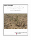
Acta Universitatis Agriculturae et Silviculturae Mendelianae Brunensis, 2014
Download

Vegetable Crops Research Bulletin, 2000
Download

HortScience
Download

Journal of Fruit and Ornamental Plant Research, 2010
Download

Journal of the ASFMRA, 2009
Download


Prace Komisji Kultury Słowian, 2022
Download


Download