Entropy Production and Time Asymmetry in Nonequilibrium Fluctuations

Entropy production and time asymmetry in nonequilibrium fluctuations D. Andrieux and P. Gaspard arXiv:cond-mat/0703696v2 [cond-mat.stat-mech] 3 May 2007 Center for Nonlinear Phenomena and Complex Systems, Université Libre de Bruxelles, Code Postal 231, Campus Plaine, B-1050 Brussels, Belgium S. Ciliberto, N. Garnier, S. Joubaud, and A. Petrosyan Laboratoire de Physique, CNRS UMR 5672, Ecole Normale Supérieure de Lyon, 46 Allée d’Italie, 69364 Lyon Cédex 07, France The time-reversal symmetry of nonequilibrium fluctuations is experimentally investigated in two out-of-equilibrium systems namely, a Brownian particle in a trap moving at constant speed and an electric circuit with an imposed mean current. The dynamical randomness of their nonequilibrium fluctuations is characterized in terms of the standard and time-reversed entropies per unit time of dynamical systems theory. We present experimental results showing that their difference equals the thermodynamic entropy production in units of Boltzmann’s constant. PACS numbers: 05.70.Ln; 05.40.-a; 02.50.Ey Newton’s equations ruling the motion of particles in matter are known to be time-reversal symmetric. Yet, macroscopic processes present irreversible behavior in which entropy is produced according to the second law of thermodynamics. Recent works suggest that this thermodynamic time asymmetry could be understood in terms similar as those used for other symmetry breaking phenomena in condensed matter physics. The breaking of time-reversal symmetry should concern the fluctuations in systems driven out of equilibrium. These fluctuations may be described in terms of the probabilities weighting the different possible trajectories of the systems. Albeit the time-reversal symmetry of the microscopic Newtonian dynamics says that each trajectory corresponds to a time-reversed one, it turns out that distinct forward and backward trajectories may have different probability weights if the system is out of equilibrium. For example, the probability for a driven Brownian particle of having a trajectory from a point A to a point B is different of having the same reverse trajectory from B to A. This important observation can be further elaborated to establish a connection with the entropy production. We consider the paths or histories z = (z0 , z1 , z2 , ..., zn−1 ) obtained by sampling the trajectories z(t) at regular time intervals τ . The probability weight of a typical path is known to decay as P+ (z0 , z1 , z2 , ..., zn−1 ) ∼ exp(−nτ h) (1) as the number n of time intervals increases [1, 2, 3, 4]. The decay rate h is called the entropy per unit time and it characterizes the temporal disorder, i.e., dynamical randomness, in both deterministic dynamical systems and stochastic processes [1, 2, 3, 4]. We can compare (1) with the probability weight of the time-reversed path zR = (zn−1 , ..., z2 , z1 , z0 ) in the nonequilibrium system with reversed driving constraints (denoted by the minus sign): P− (zn−1 , ..., z2 , z1 , z0 ) ∼ exp(−nτ hR ) . (2) It can be shown that, out of equilibrium, the probabilities of the time-reversed paths decay faster than the probabilities of the paths themselves [5]. We may interpret this as a breaking of the time-reversal symmetry in the invariant probability distribution describing the nonequilibrium steady state, the fundamental underlying Newtonian dynamics still being time-reversal symmetric. The decay rate hR in Eq. (2) is called the time-reversed entropy per unit time and characterizes the dynamical randomness of the time-reversed paths [5, 6]. In the case of Markovian stochastic processes with discrete fluctuating variables, the difference between both quantities hR and h gives the entropy production of irreversible thermodynamics [5, 6, 7, 8]. A closely related result has been obtained for the work dissipated in transient timedependent systems [9]. However, many experimental systems have continuous fluctuating variables and evolve in nonequilibrium steady states. Therefore, we may wonder how to measure dynamical randomness in such systems of experimental interest and whether the time asymmetry of this property can be experimentally detected and related to the thermodynamic entropy production. In the present Letter, we provide experimental evidence for the aforementioned time asymmetry in two nonequilibrium systems, namely, a driven Brownian motion and a fluctuating electric circuit. For this purpose, the decay rates h and hR are considered as socalled (ǫ, τ )-entropies per unit time, which characterize dynamical randomness in continuous-variable stochastic processes [4]. These entropies per unit time can be obtained by applying to the present stochastic systems a method originally proposed for the study of deterministic dynamical systems [1, 2, 3]. Thanks to this method, the (ǫ, τ )-entropies per unit time of the paths and the corresponding time-reversed paths can be evaluated from two long time series measured with sufficient temporal and spatial resolutions, in two similar runs but one driven with an opposite nonequilibrium constraint. The experiment thus consists in recording a pair of long time series 2 in each system. The dissipated heat and thermodynamic entropy production are thus given by the difference between the two (ǫ, τ )-entropies per unit time. The first system is a Brownian particle dragged by an optical tweezer, which is composed by a large aperture microscope objective (×63, 1.3) and by an infrared laser beam with a wavelength of 980 nm and a power of 20 mW on the focal plane. The trapped polystyrene particle has a diameter of 2 µm and is suspended in a 20% glycerol-water solution. The particle is trapped at 20 µm from the bottom plate of the cell which is 200 µm thick. The detection of the particle position xt is done using a He-Ne laser and an interferometric technique [10]. In order to apply a shear to the trapped particle, the cell is moved with a feedback-controlled piezo which insures a perfect linearity of displacement. The motion of the dragged particle is overdamped and can be modeled as the Langevin equation α dxt = F (xt − ut) + ξ(t) , dt (3) where α is the viscous friction coefficient, F = −∂x V is the force exerted by the potential V = kx2 /2 of the laser trap moving at constant velocity u, and ξ(t) a Gaussian white noise [11]. The stiffness of the potential is k = 9.62 10−6 kg s−2 . The relaxation time is τR = α/k = 3.05 10−3 s. The second system is an electric circuit driven out of equilibrium by a current source which imposes the mean current I [12]. The current fluctuates in the circuit because of the intrinsic Nyquist thermal noise [11]. The electric circuit is composed of a capacitance C = 278 pF in parallel with a resistance R = 9.22 MΩ so that the time constant of the circuit is τR = RC = 2.56 10−3 s. This electric circuit and the dragged Brownian particle, although physically different, are known to be formally equivalent by the correspondence α ↔ R, k ↔ 1/C and u ↔ I while the particle position xt corresponds to the charge qt inside the resistor at time t [11, 12]. The variables xt and qt are acquired at a sampling frequency 1/τ = 8192 Hz. In both experiments, the temperature is T = 298 K. In order to fix the ideas, we describe our method in the case of the dragged Brownian particle. The heat dissipated along a random trajectory during a time interval t is given by [11, 13] Z t dxt′ (4) F (xt′ − ut′ ) dt′ . Qt = ′ dt 0 After a long enough time, the system reaches a nonequilibrium steady state, in which the entropy production is related to the mean value of the dissipated heat according to 1 dhQt i αu2 di S = = . dt T dt T (5) Our aim is to show that one can extract the heat dissipated along a fluctuating path by comparing the probability of this path, with the one of the time-reversed path having also reversed the displacement of the potential, i.e., u → −u. We first make the change to the frame comoving with the minimum of the potential so that z ≡ x − ut. After initial transients, the system will reach a steady state characterized by a stationary probability distribution. As we are interested in the probability of a given succession of states corresponding to a discretization of the signal at small time intervals τ , a multi-time random variable is defined according to Z = [Z(t0 ), Z(t0 + τ ), . . . , Z(t0 + nτ − τ )] which corresponds to the signal during the time period t − t0 = nτ . For a stationary process their distribution do not depend on the initial time t0 . From the point of view of probability theory, the process is defined by the n-time joint probabilities Pσ (z; dz, τ, n) = Pr{z < Z < z+dz; σ} = pσ (z)dz, where pσ (z) is the probability density for Z to take the value z = (z0 , z1 , . . . , zn−1 ) at times t0 + iτ for a nonequilibrium driving σ = u/|u| = ±1. Since the process is Markovian, the joint probabilities can be decomposed into the products of the Green functions G(zi , zi−1 ; τ )dzi for i = 1, . . . , n. G(z, z0 ; t) gives the probability density for the position to be z at time t given that the initial position was z0 [14, 15]. To extract the dissipation occurring along a single trajectory, one has to look at the ratio of the probability of the forward path over the probability of the reversed path having also reversed the displacement of the potential. Indeed, taking the logarithm of this ratio and the continuous limit τ → 0, n → ∞ with nτ = t, we find ln P+ (z; dz, τ, n) = βu P− (zR ; dz, τ, n) Z 0 t h i F (zt′ ) dt′ −β V (zt )−V (z0 ) (6) which is exactly the heat Qt in Eq. (4) expressed in the z variable and multiplied by the inverse temperature β = (kB T )−1 . We notice that, alone, the first term gives the work exerted by the trap [13, 16]. Relations similar to Eq. (6) have been obtained for the distribution of the work done on a time-dependent system [17, 18] and for Boltzmann’s entropy production [19]. We emphasize that Eq. (6) also holds for anharmonic potentials V and that the reversal of u is essential to get the dissipated heat from the way the path probabilities P+ and P− differ. Now, due to the continuous nature in time and in space of the process, one has to consider (ǫ, τ ) quantities, i.e. quantities defined on cells of size ǫ and measured at time intervals τ . Therefore, we introduce the probability P+ (Zm ; ǫ, τ, n) for the path to remain within a distance ǫ of some reference path Zm , made of n successive positions of the Brownian particle observed at time intervals τ for the forward process. The probability is obtained by searching for the recurrences of M such reference paths 3 20 100 (a) 15 z (nm) H(ε,τ,n) 50 10 5 0 0 0 −50 0.001 0.002 nτ (s) 0.003 0.004 0.001 0.002 nτ (s) 0.003 0.004 0.001 0.002 nτ (s) 0.003 0.004 14 (b) 12 0.9 1 0.95 H R(ε,τ,n) 10 −100 1.05 time (s) 8 6 4 2 FIG. 1: Time series of typical paths z(t) for the Brownian particle in the optical trap moving at the velocity u for the forward process (upper curve) and −u for the reversed process (lower curve) with u = 4.24 10−6 m/s. 0 0 1 2 3 4 5 6 7 8 9 10 11 12 13 14 15 16 17 18 19 20 1.2 (c) 1.1 H(ǫ, τ, n) = − M 1 X ln P+ (Zm ; ǫ, τ, n) M m=1 (7) H R−H 1 or patterns in the time series. Next, we also introduce the probability P− (ZR m ; ǫ, τ, n) for a reversed path of the reversed process to remain within a distance ǫ of the reference path Zm (of the forward process) during n successive positions. 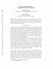According to a numerical procedure proposed by Grassberger, Procaccia and others [1, 2] the entropy per unit time can be estimated by the linear growth of the mean ‘pattern entropy’ defined as 0.9 0.8 0.7 0.6 0 FIG. 2: (a) Entropy production of the Brownian particle versus the driving speed u. The solid line is given by Eq. (5). (b) Entropy production of the RC electric circuit versus the injected current I. The solid line is the Joule law, di S/dt = RI 2 /T . The dots are the results of Eq. (9). By similarity, we introduce H R (ǫ, τ, n) = − M 1 X ln P− (ZR m ; ǫ, τ, n) M m=1 (8) for the reversed process. The (ǫ,τ )-entropies per unit time, h(ǫ, τ ) and hR (ǫ, τ ), are defined by the linear growth of these mean pattern entropies as a function of the time nτ [1, 2, 4]. In the nonequilibrium steady state, the thermodynamic entropy production should thus be given by the difference between these two quantities: 1 di S = lim lim [hR (ǫ, τ ) − h(ǫ, τ )] . ǫ→0 τ →0 kB dt (9) It is important to note that the probabilities of the reversed paths are averaged over the paths of the forward process in order for Eq. (9) to hold. The entropy production is thus expressed as the difference of two usually very large quantities which increase with the scaling law ǫ−2 for ǫ, τ going to zero [4, 20]. Nevertheless, their difference remains finite and gives the entropy production in terms of the time asymmetry of the dynamical randomness characterized by the (ǫ,τ )-entropies per unit time. In order to test experimentally that entropy production is related to this time asymmetry according to Eq. (9), we have analyzed for specific values of |u| or |I|, a pair of time series up to 2 107 points each, one corresponding to the forward process and the other corresponding to the reversed process, having first discarded the transient evolution. Figure 1 depicts examples of paths z(t) for the Brownian particle in a moving optical trap. For different values of ǫ between 5.6-11.2 nm [21], the mean pattern entropy (7) is calculated with the distance defined by taking the maximum among the deviations |Z(t) − Zm (t)| with respect to some reference path Zm for the times t = 0, τ, . . . , (n − 1)τ . The forward entropy per unit time h(ǫ, τ ) is evaluated from the linear growth of the mean pattern entropy (7) with the time nτ . The backward entropy per unit time hR (ǫ, τ ) is obtained similarly from the time-reversed pattern entropy (8). The difference of the two dynamical entropies is depicted as in Fig. 2a. The good agreement with the entropy production (5) is the experimental evidence that this latter is indeed related to the time asymmetry of dynamical randomness as predicted by Eq. (9). 4 In conclusion, we measured the entropy production by searching the recurrences of trajectories in the fluctuating dynamics of two nonequilibrium processes. The experiments we performed consisted in the recording of two long time series. The first one corresponds to a forward experiment while the other is measured from the same experimental setup except that the sign of the constraint driving the system out of equilibrium has been reversed. From these two time series, we are able to compute two dynamical entropies, the difference of which gives the entropy production. Moreover, we tested the possibility to extract the dissipated heat along a single random path. This shows that the entropy production arises from the breaking of the time-reversal symmetry in the probability distribution of the statistical description of the nonequilibrium steady state. Since the decay rates of the multitime probabilities of the forward and reversed paths characterize their dynamical randomness, the present results show that the thermodynamic entropy production finds its origin in the time asymmetry of the dynamical randomness. Acknowledgments. This research is financially supported by the F .N .R .S . Belgium and the “Communauté française de Belgique” (contract “Actions de Recherche Concertées” No. 04/09-312). [1] P. Grassberger and I. Procaccia, Phys. Rev. A 28, 2591 (1983). [2] A. Cohen and I. Procaccia, Phys. Rev. A 31, 1872 (1985). [3] J.-P. Eckmann and D. Ruelle, Rev. Mod. Phys. 57, 617 (1985). [4] P. Gaspard and X. J. Wang, Phys. Rep. 235, 291 (1993). [5] P. Gaspard, J. Stat. Phys. 117, 599 (2004). [6] P. Gaspard, New Journal of Physics 7, 77 (2005). [7] V. Lecomte, C. Appert-Rolland, and F. van Wijland, Phys. Rev. Lett. 95, 010601 (2005). [8] J. Naudts and E. Van der Straeten, Phys. Rev. E 74, (a) diS/dt (k BT/s) We also tested the possibility to extract the heat (4) dissipated along a single stochastic path by searching for the recurrences in the time series according to Eq. (6). A randomly selected path as well as the corresponding heat dissipated are plotted in Fig. 3. We find a very good agreement so that the relation (6) is also verified for single paths. In this case, the heat exchanged between the particle and the surrounding fluid can be positive or negative because of the molecular fluctuations. It is only by averaging over the forward process that the dissipated heat takes the positive value depicted in Fig. 2. 150 100 50 0 0 1 2 3 4 5 u (µm/s) 250 (b) 200 diS/dt (k BT/s) On the other hand, we have analyzed by the same method the time series of the RC electric circuit. We see in Fig. 2b that the entropy production obtained from the time series analysis of the RC circuit agrees very well with the known Joule law, which is a further confirmation of Eq. (9). 150 100 50 0 0 0.1 0.2 0.3 I (pA) FIG. 3: Measure of the heat dissipated by the Brownian particle along the forward and reversed paths of Fig. 1. The trap velocities are ±u with u = 4.24 10−6 m/s. We are searching for recurrences between the two processes. (a) Inset: A randomly selected trajectory in the time series. The probabilities of the corresponding forward (filled circles) and the backward (open circles) paths for ǫ = 8.4 nm. These probabilities present an exponential decrease modulated by the fluctuations. (b) The dissipated heat given by the logarithm of the ratio of the forward and backward probabilities according to Eq. (6) for different values of ǫ = k × 0.558 nm with k = 11, . . . , 20 in the range 6.1-11.2 nm. They are compared with the value (squares) directly calculated from Eq. (4). For small values of ǫ, the agreement is quite good for short time and within experimental errors for larger time. 040103R (2006). [9] C. Jarzynski, Phys. Rev. E 73, 046105 (2006). [10] B. Schnurr, F. Gittes, F. C. MacKintosh, and C. F. Schmidt, Macromolecules 30(25), 7781 (1997). [11] R. van Zon, S. Ciliberto and E. G. D. Cohen, Phys. Rev. Lett. 92, 130601 (2004). [12] N. Garnier and S. Ciliberto, Phys. Rev. E 71, R060101 (2005). [13] K. Sekimoto, J. Phys. Soc. Japan 66, 1234 (1997). [14] S. Chandrasekhar, Rev. Mod. Phys. 15, 1 (1943). [15] L. Onsager and S. Machlup, Phys. Rev. 91, 1505 (1953). [16] G. M. Wang, E. M. Sevick, E. Mittag, D. J. Searles, and D. J. Evans, Phys. Rev. Lett. 89, 050601 (2002). [17] G. E. Crooks, Phys. Rev. E 60, 2721 (1999). [18] B. Cleuren, C. Van den Broeck, and R. Kawai, Phys. 5 Rev. Lett. 96, 050601 (2006). [19] C. Maes and K. Netočný, J. Stat. Phys. 110, 269 (2003). [20] P. Gaspard, M. E. Briggs, M. K. Francis, J. V. Sengers, R. W. Gammon, J. R. Dorfman, and R. V. Calabrese, View publication stats Nature 394, 865 (1998). [21] We notice that the statistics is not sufficient for smaller values of ǫ, while the graining is too coarse for larger values.