VL2: A Scalable and Flexible Data Center Network
Albert Greenberg
Srikanth Kandula
David A. Maltz
James R. Hamilton
Changhoon Kim
Parveen Patel
Navendu Jain
Parantap Lahiri
Sudipta Sengupta
Microsoft Research
Abstract
Agility promises improved risk management and cost savings.
Without agility, each service must pre-allocate enough servers to
meet difficult to predict demand spikes, or risk failure at the brink
of success. With agility, the data center operator can meet the fluctuating demands of individual services from a large shared server
pool, resulting in higher server utilization and lower costs.
Unfortunately, the designs for today’s data center network prevent agility in several ways. First, existing architectures do not
provide enough capacity between the servers they interconnect.
Conventional architectures rely on tree-like network configurations
built from high-cost hardware. Due to the cost of the equipment,
the capacity between different branches of the tree is typically oversubscribed by factors of : or more, with paths through the highest
levels of the tree oversubscribed by factors of : to :. This limits communication between servers to the point that it fragments the
server pool — congestion and computation hot-spots are prevalent
even when spare capacity is available elsewhere. Second, while data
centers host multiple services, the network does little to prevent a
traffic flood in one service from affecting the other services around
it — when one service experiences a traffic flood,it is common for all
those sharing the same network sub-tree to suffer collateral damage.
Third, the routing design in conventional networks achieves scale by
assigning servers topologically significant IP addresses and dividing
servers among VLANs. Such fragmentation of the address space
limits the utility of virtual machines, which cannot migrate out of
their original VLAN while keeping the same IP address. Further,
the fragmentation of address space creates an enormous configuration burden when servers must be reassigned among services, and
the human involvement typically required in these reconfigurations
limits the speed of deployment.
To overcome these limitations in today’s design and achieve
agility, we arrange for the network to implement a familiar and
concrete model: give each service the illusion that all the servers
assigned to it, and only those servers, are connected by a single
non-interfering Ethernet switch—a Virtual Layer — and maintain
this illusion even as the size of each service varies from server to
,. Realizing this vision concretely translates into building a
network that meets the following three objectives:
To be agile and cost effective, data centers should allow dynamic resource allocation across large server pools. In particular, the data
center network should enable any server to be assigned to any service. To meet these goals, we present VL, a practical network architecture that scales to support huge data centers with uniform high
capacity between servers, performance isolation between services,
and Ethernet layer- semantics. VL uses () flat addressing to allow
service instances to be placed anywhere in the network, () Valiant
Load Balancing to spread traffic uniformly across network paths,
and () end-system based address resolution to scale to large server
pools, without introducing complexity to the network control plane.
VL’s design is driven by detailed measurements of traffic and fault
data from a large operational cloud service provider. VL’s implementation leverages proven network technologies, already available
at low cost in high-speed hardware implementations, to build a scalable and reliable network architecture. As a result, VL networks
can be deployed today, and we have built a working prototype. We
evaluate the merits of the VL design using measurement, analysis,
and experiments. Our VL prototype shuffles . TB of data among
servers in seconds – sustaining a rate that is of the maximum possible.
Categories and Subject Descriptors: C.. [Computer-Communication Network]: Network Architecture and Design
General Terms: Design, Performance, Reliability
Keywords: Data center network, commoditization
1. INTRODUCTION
Cloud services are driving the creation of data centers that hold
tens to hundreds of thousands of servers and that concurrently support a large number of distinct services (e.g., search, email, mapreduce computations, and utility computing). The motivations for
building such shared data centers are both economic and technical:
to leverage the economies of scale available to bulk deployments and
to benefit from the ability to dynamically reallocate servers among
services as workload changes or equipment fails [, ]. The cost is
also large – upwards of million per month for a , server
data center — with the servers themselves comprising the largest
cost component. To be profitable, these data centers must achieve
high utilization, and key to this is the property of agility — the capacity to assign any server to any service.
• Uniform high capacity: The maximum rate of a server-to-server
traffic flow should be limited only by the available capacity on the
network-interface cards of the sending and receiving servers, and
assigning servers to a service should be independent of network
topology.
• Performance isolation: Traffic of one service should not be affected by the traffic of any other service, just as if each service was
connected by a separate physical switch.
Permission to make digital or hard copies of all or part of this work for
personal or classroom use is granted without fee provided that copies are
not made or distributed for profit or commercial advantage and that copies
bear this notice and the full citation on the first page. To copy otherwise, to
republish, to post on servers or to redistribute to lists, requires prior specific
permission and/or a fee.
SIGCOMM’09, August 17–21, 2009, Barcelona, Spain.
Copyright 2009 ACM 978-1-60558-594-9/09/08 ...$10.00.
• Layer- semantics: Just as if the servers were on a LAN—where
any IP address can be connected to any port of an Ethernet switch
due to flat addressing—data-center management software should
be able to easily assign any server to any service and configure
51
�✂✄
✂
✂✄
✂
✁
☎
✁
✄
✁
☎
✁
✄
✆
✝ ✆
✝
☞
✡
✂
✂✄
☛
☛
✄
✁
☎
✌
☛
✄
☎✎ ✞
✍
✝ ✞
✝✟
✞
✝ ✞
✝
✌
☛
✄
☎✑ ✞
✍
✠ ✞
✠
✦
✧
★
✙
✬
✪
✪
✮✘
✤
✜
✘
✤
✭
✜
✫
✩
•✩
✒
✙
✬
✒
✪
✪
✮
✯
✯
✘
✰
✰
✤
✭
✘
✜
✫
•
✠ ✠ ✠ ✠✟
✲
✒
✓✙
✢
✒
✓
✔✮✯
✖
✜
✱
• ✫✖
✲
✓
✙
✢
✓
✔
✮
✯
• ✫✱
✶✵✪
✷
✲
✓
✔✮✯
✪
✤
✤
✴
✚
✯
✱
✫
✵✤
✸
✺ ✸
✺✸
✺ ✸
✺ •✳
✳
✹
✹
✹
✹
✻✼✽✾✼✽✿✏
✻✼✽✾✼✽✿ ✻✼✽✾✼✽✿✏
✻✼✽✾✼✽✿
✗✘
✒
✓
✔✕
✙
✔✕
✣
✖
✚
✛
✘
✜✢
✤
✥
✚
that server with whatever IP address the service expects. Virtual
machines should be able to migrate to any server while keeping
the same IP address, and the network configuration of each server
should be identical to what it would be if connected via a LAN.
Finally, features like link-local broadcast, on which many legacy
applications depend, should work.
In this paper we design, implement and evaluate VL, a network architecture for data centers that meets these three objectives
and thereby provides agility. In creating VL, a goal was to investigate whether we could create a network architecture that could be
deployed today, so we limit ourselves from making any changes to
the hardware of the switches or servers, and we require that legacy
applications work unmodified. However, the software and operating systems on data-center servers are already extensively modified
(e.g., to create hypervisors for virtualization or blob file-systems to
store data). Therefore, VL’s design explores a new split in the responsibilities between host and network — using a layer . shim
in servers’ network stack to work around limitations of the network
devices. No new switch software or APIs are needed.
VL consists of a network built from low-cost switch ASICs
arranged into a Clos topology [] that provides extensive path diversity between servers. Our measurements show data centers have
tremendous volatility in their workload, their traffic, and their failure patterns. To cope with this volatility, we adopt Valiant Load
Balancing (VLB) [, ] to spread traffic across all available paths
without any centralized coordination or traffic engineering. Using
VLB, each server independently picks a path at random through the
network for each of the flows it sends to other servers in the data
center. Common concerns with VLB, such as the extra latency and
the consumption of extra network capacity caused by path stretch,
are overcome by a combination of our environment (propagation
delay is very small inside a data center) and our topology (which
includes an extra layer of switches that packets bounce off of). Our
experiments verify that our choice of using VLB achieves both the
uniform capacity and performance isolation objectives.
The switches that make up the network operate as layer-
routers with routing tables calculated by OSPF, thereby enabling the
use of multiple paths (unlike Spanning Tree Protocol) while using a
well-trusted protocol. However, the IP addresses used by services
running in the data center cannot be tied to particular switches
in the network, or the agility to reassign servers between services
would be lost. Leveraging a trick used in many systems [], VL
assigns servers IP addresses that act as names alone, with no topological significance. When a server sends a packet, the shim-layer
on the server invokes a directory system to learn the actual location
of the destination and then tunnels the original packet there. The
shim-layer also helps eliminate the scalability problems created by
ARP in layer- networks, and the tunneling improves our ability to
implement VLB. These aspects of the design enable VL to provide
layer- semantics, while eliminating the fragmentation and waste of
server pool capacity that the binding between addresses and locations causes in the existing architecture.
Taken together, VL’s choices of topology, routing design, and
software architecture create a huge shared pool of network capacity
that each pair of servers can draw from when communicating. We
implement VLB by causing the traffic between any pair of servers
to bounce off a randomly chosen switch in the top level of the Clos
topology and leverage the features of layer- routers, such as EqualCost MultiPath (ECMP), to spread the traffic along multiple subpaths for these two path segments. Further, we use anycast addresses
and an implementation of Paxos [] in a way that simplifies the
design of the Directory System and, when failures occur, provides
consistency properties that are on par with existing protocols.
Figure : A conventional network architecture for data centers
(adapted from figure by Cisco []).
The feasibility of our design rests on several questions that we
experimentally evaluate. First, the theory behind Valiant Load Balancing, which proves that the network will be hot-spot free, requires
that (a) randomization is performed at the granularity of small packets, and (b) the traffic sent into the network conforms to the hose
model []. For practical reasons, however, VL picks a different
path for each flow rather than packet (falling short of (a)), and it
also relies on TCP to police the offered traffic to the hose model
(falling short of (b), as TCP needs multiple RTTs to conform traffic to the hose model). Nonetheless, our experiments show that for
data-center traffic, the VL design choices are sufficient to offer the
desired hot-spot free properties in real deployments. Second, the
directory system that provides the routing information needed to
reach servers in the data center must be able to handle heavy workloads at very low latency. We show that designing and implementing
such a directory system is achievable.
In the remainder of this paper we will make the following contributions, in roughly this order.
• We make a first of its kind study of the traffic patterns in a production data center, and find that there is tremendous volatility in the
traffic, cycling among - different patterns during a day and
spending less than s in each pattern at the th percentile.
• We design, build, and deploy every component of VL in an server cluster. Using the cluster, we experimentally validate that
VL has the properties set out as objectives, such as uniform capacity and performance isolation. We also demonstrate the speed
of the network, such as its ability to shuffle . TB of data among
servers in s.
• We apply Valiant Load Balancing in a new context, the interswitch fabric of a data center, and show that flow-level traffic splitting achieves almost identical split ratios (within of optimal
fairness index) on realistic data center traffic, and it smoothes utilization while eliminating persistent congestion.
• We justify the design trade-offs made in VL by comparing the
cost of a VL network with that of an equivalent network based
on existing designs.
2. BACKGROUND
In this section, we first explain the dominant design pattern for
data-center architecture today []. We then discuss why this architecture is insufficient to serve large cloud-service data centers.
As shown in Figure , the network is a hierarchy reaching from
a layer of servers in racks at the bottom to a layer of core routers at
the top. There are typically to servers per rack, each singly connected to a Top of Rack (ToR) switch with a Gbps link. ToRs connect to two aggregation switches for redundancy, and these switches
aggregate further connecting to access routers. At the top of the hierarchy, core routers carry traffic between access routers and man-
52
�PDF
age traffic into and out of the data center. All links use Ethernet as
a physical-layer protocol, with a mix of copper and fiber cabling.
All switches below each pair of access routers form a single layer domain, typically connecting several thousand servers. To limit
overheads (e.g., packet flooding and ARP broadcasts) and to isolate different services or logical server groups (e.g., email, search,
web front ends, web back ends), servers are partitioned into virtual LANs (VLANs). Unfortunately, this conventional design suffers
from three fundamental limitations:
Limited server-to-server capacity: As we go up the hierarchy, we are confronted with steep technical and financial barriers
in sustaining high bandwidth. Thus, as traffic moves up through the
layers of switches and routers, the over-subscription ratio increases
rapidly. For example, servers typically have : over-subscription to
other servers in the same rack — that is, they can communicate at
the full rate of their interfaces (e.g., Gbps). We found that up-links
from ToRs are typically : to : oversubscribed (i.e., to Gbps
of up-link for servers), and paths through the highest layer of
the tree can be : oversubscribed. This large over-subscription
factor fragments the server pool by preventing idle servers from being assigned to overloaded services, and it severely limits the entire
data-center’s performance.
Fragmentation of resources: As the cost and performance of
communication depends on distance in the hierarchy, the conventional design encourages service planners to cluster servers nearby
in the hierarchy. Moreover, spreading a service outside a single
layer- domain frequently requires reconfiguring IP addresses and
VLAN trunks, since the IP addresses used by servers are topologically determined by the access routers above them. The result is
a high turnaround time for such reconfiguration. Today’s designs
avoid this reconfiguration lag by wasting resources; the plentiful
spare capacity throughout the data center is often effectively reserved by individual services (and not shared), so that each service
can scale out to nearby servers to respond rapidly to demand spikes
or to failures. Despite this, we have observed instances when the
growing resource needs of one service have forced data center operations to evict other services from nearby servers, incurring significant cost and disruption.
Poor reliability and utilization: Above the ToR, the basic resilience model is :, i.e., the network is provisioned such that if an
aggregation switch or access router fails, there must be sufficient remaining idle capacity on a counterpart device to carry the load. This
forces each device and link to be run up to at most of its maximum utilization. Further, multiple paths either do not exist or aren’t
effectively utilized. Within a layer- domain, the Spanning Tree Protocol causes only a single path to be used even when multiple paths
between switches exist. In the layer- portion, Equal Cost Multipath
(ECMP) when turned on, can use multiple paths to a destination
if paths of the same cost are available. However, the conventional
topology offers at most two paths.
0.45
0.4
0.35
0.3
0.25
0.2
0.15
0.1
0.05
0
Flow Size PDF
Total Bytes PDF
1
100
10000 1e+06 1e+08 1e+10 1e+12
CDF
Flow Size (Bytes)
1
0.8
0.6
0.4
0.2
0
Flow Size CDF
Total Bytes CDF
1
100
10000 1e+06 1e+08 1e+10 1e+12
Flow Size (Bytes)
Figure : Mice are numerous; of flows are smaller than
MB. However, more than of bytes are in flows between
MB and GB.
Our measurement studies found two key results with implications for the network design. First, the traffic patterns inside a data
center are highly divergent (as even over representative traffic
matrices only loosely cover the actual traffic matrices seen),and they
change rapidly and unpredictably. Second, the hierarchical topology
is intrinsically unreliable—even with huge effort and expense to increase the reliability of the network devices close to the top of the
hierarchy, we still see failures on those devices resulting in significant downtimes.
3.1 Data-Center Traffic Analysis
Analysis of Netflow and SNMP data from our data centers reveals several macroscopic trends. First, the ratio of traffic volume
between servers in our data centers to traffic entering/leaving our
data centers is currently around : (excluding CDN applications).
Second, data-center computation is focused where high speed access to data on memory or disk is fast and cheap. Although data
is distributed across multiple data centers, intense computation and
communication on data does not straddle data centers due to the
cost of long-haul links. Third, the demand for bandwidth between
servers inside a data center is growing faster than the demand for
bandwidth to external hosts. Fourth, the network is a bottleneck
to computation. We frequently see ToR switches whose uplinks are
above utilization.
To uncover the exact nature of traffic inside a data center, we
instrumented a highly utilized , node cluster in a data center
that supports data mining on petabytes of data. The servers are
distributed roughly evenly across ToR switches, which are connected hierarchically as shown in Figure . We collected socket-level
event logs from all machines over two months.
3.2 Flow Distribution Analysis
3. MEASUREMENTS & IMPLICATIONS
Distribution of flow sizes: Figure illustrates the nature of
flows within the monitored data center. The flow size statistics
(marked as ‘+’s) show that the majority of flows are small (a few
KB); most of these small flows are hellos and meta-data requests to
the distributed file system. To examine longer flows, we compute a
statistic termed total bytes (marked as ‘o’s) by weighting each flow
size by its number of bytes. Total bytes tells us, for a random byte,
the distribution of the flow size it belongs to. Almost all the bytes
in the data center are transported in flows whose lengths vary from
about MB to about GB. The mode at around MB springs
from the fact that the distributed file system breaks long files into
-MB size chunks. Importantly, flows over a few GB are rare.
To design VL, we first needed to understand the data center environment in which it would operate. Interviews with architects, developers, and operators led to the objectives described in
Section , but developing the mechanisms on which to build the
network requires a quantitative understanding of the traffic matrix
(who sends how much data to whom and when?) and churn (how
often does the state of the network change due to changes in demand
or switch/link failures and recoveries, etc.?). We analyze these aspects by studying production data centers of a large cloud service
provider and use the results to justify our design choices as well as
the workloads used to stress the VL testbed.
53
�1000
Number of Concurrent flows in/out of each Machine
15
10
300
200
200
5
0
Figure : Number of concurrent connections has two modes: ()
flows per node more than of the time and () flows per
node for at least of the time.
Frequency
100
20
100
10
25
0
200 400 600 800 1000
Time in 100s intervals
(a)
0
1
Frequency
0
30
50 100
0.01
35
0
0.02
40
Index of the Containing Cluster
1
0.8
0.6
0.4
0.2
0
PDF
CDF
0.03
Cumulative
Fraction of Time
0.04
0
5 10
Run Length
(b)
20
2.0
3.0
4.0
log(Time to Repeat)
(c)
Figure : Lack of short-term predictability: The cluster to which
a traffic matrix belongs, i.e., the type of traffic mix in the TM,
changes quickly and randomly.
Similar to Internet flow characteristics [], we find that there are
myriad small flows (mice). On the other hand, as compared with
Internet flows, the distribution is simpler and more uniform. The
reason is that in data centers, internal flows arise in an engineered
environment driven by careful design decisions (e.g., the -MB
chunk size is driven by the need to amortize disk-seek times over
read times) and by strong incentives to use storage and analytic tools
with well understood resilience and performance.
Number of Concurrent Flows: Figure shows the probability
density function (as a fraction of time) for the number of concurrent flows going in and out of a machine, computed over all ,
monitored machines for a representative day’s worth of flow data.
There are two modes. More than of the time, an average machine has about ten concurrent flows, but at least of the time it
has greater than concurrent flows. We almost never see more
than concurrent flows.
The distributions of flow size and number of concurrent flows
both imply that VLB will perform well on this traffic. Since even big
flows are only MB ( s of transmit time at Gbps), randomizing at flow granularity (rather than packet) will not cause perpetual
congestion if there is unlucky placement of a few flows. Moreover,
adaptive routing schemes may be difficult to implement in the data
center, since any reactive traffic engineering will need to run at least
once a second if it wants to react to individual flows.
Surprisingly, the number of representative traffic matrices in
our data center is quite large. On a timeseries of TMs, indicating a day’s worth of traffic in the datacenter, even when approximating with 50 − 60 clusters, the fitting error remains high () and
only decreases moderately beyond that point. This indicates that the
variability in datacenter traffic is not amenable to concise summarization and hence engineering routes for just a few traffic matrices
is unlikely to work well for the traffic encountered in practice.
Instability of traffic patterns: Next we ask how predictable is
the traffic in the next interval given the current traffic? Traffic predictability enhances the ability of an operator to engineer routing
as traffic demand changes. To analyze the predictability of traffic in
the network, we find the best TM clusters using the technique
above and classify the traffic matrix for each s interval to the
best fitting cluster. Figure (a) shows that the traffic pattern changes
nearly constantly, with no periodicity that could help predict the future. Figure (b) shows the distribution of run lengths - how many
intervals does the network traffic pattern spend in one cluster before shifting to the next. The run length is to the th percentile.
Figure (c) shows the time between intervals where the traffic maps
to the same cluster. But for the mode at s caused by transitions
within a run, there is no structure to when a traffic pattern will next
appear.
The lack of predictability stems from the use of randomness to
improve the performance of data-center applications. For example, the distributed file system spreads data chunks randomly across
servers for load distribution and redundancy. The volatility implies
that it is unlikely that other routing strategies will outperform VLB.
3.3 Traffic Matrix Analysis
Poor summarizability of traffic patterns: Next, we ask the
question: Is there regularity in the traffic that might be exploited
through careful measurement and traffic engineering? If traffic in the
DC were to follow a few simple patterns, then the network could be
easily optimized to be capacity-efficient for most traffic. To answer,
we examine how the Traffic Matrix(TM) of the , server cluster
changes over time. For computational tractability, we compute the
ToR-to-ToR TM — the entry T M (t)i,j is the number of bytes sent
from servers in ToR i to servers in ToR j during the s beginning
at time t. We compute one TM for every s interval, and servers
outside the cluster are treated as belonging to a single “ToR”.
Given the timeseries of TMs, we find clusters of similar TMs
using a technique due to Zhang et al. []. In short, the technique
recursively collapses the traffic matrices that are most similar to each
other into a cluster, where the distance (i.e., similarity) reflects how
much traffic needs to be shuffled to make one TM look like the
other. We then choose a representative TM for each cluster, such
that any routing that can deal with the representative TM performs
no worse on every TM in the cluster. Using a single representative
TM per cluster yields a fitting error (quantified by the distances between each representative TMs and the actual TMs they represent),
which will decrease as the number of clusters increases. Finally, if
there is a knee point (i.e., a small number of clusters that reduces
the fitting error considerably), the resulting set of clusters and their
representative TMs at that knee corresponds to a succinct number
of distinct traffic matrices that summarize all TMs in the set.
3.4 Failure Characteristics
To design VL to tolerate the failures and churn found in data
centers, we collected failure logs for over a year from eight production data centers that comprise hundreds of thousands of servers,
host over a hundred cloud services and serve millions of users. We
analyzed hardware and software failures of switches, routers, load
balancers, firewalls, links and servers using SNMP polling/traps,
syslogs, server alarms, and transaction monitoring frameworks. In
all, we looked at M error events from over K alarm tickets.
What is the pattern of networking equipment failures? We
define a failure as the event that occurs when a system or component is unable to perform its required function for more than s.
As expected, most failures are small in size (e.g., of network
device failures involve < devices and of network device failures involve < devices) while large correlated failures are rare
(e.g., the largest correlated failure involved switches). However,
downtimes can be significant: of failures are resolved in min,
in < hr, . in < day, but . last > days.
What is the impact of networking equipment failure? As discussed in Section , conventional data center networks apply : re-
54
�Separating names from locators: The data center network
must support agility, which means, in particular, support for hosting
any service on any server, for rapid growing and shrinking of server
pools, and for rapid virtual machine migration. In turn, this calls
for separating names from locations. VL’s addressing scheme separates server names, termed application-specific addresses (AAs),
from their locations, termed location-specific addresses (LAs). VL
uses a scalable, reliable directory system to maintain the mappings
between names and locators. A shim layer running in the network
stack on every server, called the VL agent, invokes the directory
system’s resolution service. We evaluate the performance of the directory system in §..
Embracing End Systems: The rich and homogeneous programmability available at data-center hosts provides a mechanism
to rapidly realize new functionality. For example, the VL agent enables fine-grained path control by adjusting the randomization used
in VLB. The agent also replaces Ethernet’s ARP functionality with
queries to the VL directory system. The directory system itself is
also realized on servers, rather than switches, and thus offers flexibility, such as fine-grained, context-aware server access control and
dynamic service re-provisioning.
We next describe each aspect of the VL system and how they
work together to implement a virtual layer- network. These aspects
include the network topology, the addressing and routing design,
and the directory that manages name-locator mappings.
Internet
Link-state network
carrying only LAs
(e.g., 10/8)
DA/2 x Intermediate Switches
...
Int
DI x10G
DA/2 x 10G
...
Aggr
DI x Aggregate Switches
DA/2 x 10G
2 x10G
...
DADI/4 x ToR Switches
ToR
❀❁
❂❃❄❅❃❄❆
20(DADI/4) x Servers
....
Fungible pool of
servers owning AAs
(e.g., 20/8)
Figure : An example Clos network between Aggregation and Intermediate switches provides a richly-connected backbone wellsuited for VLB. The network is built with two separate address
families — topologically significant Locator Addresses (LAs) and
flat Application Addresses (AAs).
dundancy to improve reliability at higher layers of the hierarchical
tree. Despite these techniques, we find that in . of failures all
redundant components in a network device group became unavailable (e.g., the pair of switches that comprise each node in the conventional network (Figure ) or both the uplinks from a switch). In
one incident, the failure of a core switch (due to a faulty supervisor card) affected ten million users for about four hours. We found
the main causes of these downtimes are network misconfigurations,
firmware bugs, and faulty components (e.g., ports). With no obvious way to eliminate all failures from the top of the hierarchy, VL’s
approach is to broaden the topmost levels of the network so that the
impact of failures is muted and performance degrades gracefully,
moving from : redundancy to n:m redundancy.
4.1 Scale-out Topologies
As described in §., conventional hierarchical data-center
topologies have poor bisection bandwidth and are also susceptible to major disruptions due to device failures at the highest levels.
Rather than scale up individual network devices with more capacity and features, we scale out the devices — build a broad network
offering huge aggregate capacity using a large number of simple, inexpensive devices, as shown in Figure . This is an example of a
folded Clos network [] where the links between the Intermediate switches and the Aggregation switches form a complete bipartite graph. As in the conventional topology, ToRs connect to two
Aggregation switches, but the large number of paths between every two Aggregation switches means that if there are n Intermediate switches, the failure of any one of them reduces the bisection
bandwidth by only 1/n–a desirable graceful degradation of bandwidth that we evaluate in §.. Further, it is easy and less expensive to build a Clos network for which there is no over-subscription
(further discussion on cost is in §). For example, in Figure , we
use DA -port Aggregation and DI -port Intermediate switches, and
connect these switches such that the capacity between each layer is
DI DA /2 times the link capacity.
The Clos topology is exceptionally well suited for VLB in that by
indirectly forwarding traffic through an Intermediate switch at the
top tier or “spine” of the network, the network can provide bandwidth guarantees for any traffic matrices subject to the hose model.
Meanwhile, routing is extremely simple and resilient on this topology — take a random path up to a random intermediate switch and
a random path down to a destination ToR switch.
VL leverages the fact that at every generation of technology, switch-to-switch links are typically faster than server-to-switch
links, and trends suggest that this gap will remain. Our current design uses G server links and G switch links, and the next design
point will probably be G server links with G switch links. By
leveraging this gap, we reduce the number of cables required to implement the Clos (as compared with a fat-tree []), and we simplify
the task of spreading load over the links (§.).
4. VIRTUAL LAYER TWO NETWORKING
Before detailing our solution, we briefly discuss our design principles and preview how they will be used in the VL design.
Randomizing to Cope with Volatility: VL copes with
the high divergence and unpredictability of data-center traffic
matrices by using Valiant Load Balancing to do destinationindependent (e.g., random) traffic spreading across multiple intermediate nodes. We introduce our network topology suited for VLB
in §., and the corresponding flow spreading mechanism in §..
VLB, in theory, ensures a non-interfering packet switched network [], the counterpart of a non-blocking circuit switched network, as long as (a) traffic spreading ratios are uniform, and (b) the
offered traffic patterns do not violate edge constraints (i.e., line card
speeds). To meet the latter condition, we rely on TCP’s end-to-end
congestion control mechanism. While our mechanisms to realize
VLB do not perfectly meet either of these conditions, we show in
§. that our scheme’s performance is close to the optimum.
Building on proven networking technology: VL is based on
IP routing and forwarding technologies that are already available
in commodity switches: link-state routing, equal-cost multi-path
(ECMP) forwarding, IP anycasting, and IP multicasting. VL uses
a link-state routing protocol to maintain the switch-level topology,
but not to disseminate end hosts’ information. This strategy protects
switches from needing to learn voluminous, frequently-changing
host information. Furthermore, the routing design uses ECMP forwarding along with anycast addresses to enable VLB with minimal
control plane messaging or churn.
55
�tory service can enforce access-control policies. Further, since the
directory system knows which server is making the request when
handling a lookup, it can enforce fine-grained isolation policies. For
example, it could enforce the policy that only servers belonging to
the same service can communicate with each other. An advantage of
VL is that, when inter-service communication is allowed, packets
flow directly from a source to a destination, without being detoured
to an IP gateway as is required to connect two VLANs in the conventional architecture.
These addressing and forwarding mechanisms were chosen for
two reasons. First, they make it possible to use low-cost switches,
which often have small routing tables (typically just 16K entries)
that can hold only LA routes, without concern for the huge number
of AAs. Second, they reduce overhead in the network control plane
by preventing it from seeing the churn in host state, tasking it to the
more scalable directory system instead.
Link-state network with LAs (10/8)
Int
(10.1.1.1)
...
H(ft)
10.1.1.1
H(ft)
10.0.0.6
20.0.0.55
20.0.0.56
Payload
(10.0.0.4)
Int
(10.1.1.1)
Int
...
(10.1.1.1)
H(ft)
10.0.0.6
20.0.0.55
20.0.0.56
Payload
(10.0.0.6)
ToR
ToR
(20.0.0.1)
(20.0.0.1)
H(ft)
10.1.1.1
H(ft)
10.0.0.6
20.0.0.55
20.0.0.56
Payload
20.0.0.55
20.0.0.66
Payload
S (20.0.0.55)
IP subnet with AAs (20/8)
D (20.0.0.56)
IP subnet with AAs (20/8)
Figure : VLB in an example VL network. Sender S sends packets to destination D via a randomly-chosen intermediate switch
using IP-in-IP encapsulation. AAs are from 20/8, and LAs are
from 10/8. H(ft) denotes a hash of the five tuple.
4.2 VL2 Addressing and Routing
4.2.2 Random traffic spreading over multiple paths
This section explains how packets flow through a VL network,
and how the topology, routing design, VL agent, and directory system combine to virtualize the underlying network fabric — creating
the illusion that hosts are connected to a big, non-interfering datacenter-wide layer- switch.
To offer hot-spot-free performance for arbitrary traffic matrices, VL uses two related mechanisms: VLB and ECMP. The goals
of both are similar — VLB distributes traffic across a set of intermediate nodes and ECMP distributes across equal-cost paths — but
each is needed to overcome limitations in the other. VL uses flows,
rather than packets, as the basic unit of traffic spreading and thus
avoids out-of-order delivery.
Figure illustrates how the VL agent uses encapsulation to implement VLB by sending traffic through a randomly-chosen Intermediate switch. The packet is first delivered to one of the Intermediate switches, decapsulated by the switch, delivered to the ToR’s LA,
decapsulated again, and finally sent to the destination.
While encapsulating packets to a specific, but randomly chosen,
Intermediate switch correctly realizes VLB, it would require updating a potentially huge number of VL agents whenever an Intermediate switch’s availability changes due to switch/link failures. Instead, we assign the same LA address to all Intermediate switches,
and the directory system returns this anycast address to agents upon
lookup. Since all Intermediate switches are exactly three hops away
from a source host, ECMP takes care of delivering packets encapsulated with the anycast address to any one of the active Intermediate
switches. Upon switch or link failures, ECMP will react, eliminating
the need to notify agents and ensuring scalability.
In practice, however, the use of ECMP leads to two problems.
First, switches today only support up to -way ECMP, with way ECMP being released by some vendors this year. If there are
more paths available than ECMP can use, then VL defines several
anycast addresses, each associated with only as many Intermediate
switches as ECMP can accommodate. When an Intermediate switch
fails, VL reassigns the anycast addresses from that switch to other
Intermediate switches so that all anycast addresses remain live, and
servers can remain unaware of the network churn. Second, some
inexpensive switches cannot correctly retrieve the five-tuple values
(e.g., the TCP ports) when a packet is encapsulated with multiple IP
headers. Thus, the agent at the source computes a hash of the fivetuple values and writes that value into the source IP address field,
which all switches do use in making ECMP forwarding decisions.
The greatest concern with both ECMP and VLB is that if “elephant flows” are present, then the random placement of flows could
lead to persistent congestion on some links while others are underutilized. Our evaluation did not find this to be a problem on datacenter workloads (§.). Should it occur, initial results show the VL
agent can detect and deal with such situations with simple mechanisms, such as re-hashing to change the path of large flows when
TCP detects a severe congestion event (e.g., a full window loss).
4.2.1 Address resolution and packet forwarding
VL uses two different IP-address families, as illustrated in Figure . The network infrastructure operates using location-specific
IP addresses (LAs); all switches and interfaces are assigned LAs, and
switches run an IP-based (layer-) link-state routing protocol that
disseminates only these LAs. This allows switches to obtain the complete switch-level topology, as well as forward packets encapsulated
with LAs along shortest paths. On the other hand, applications use
application-specific IP addresses (AAs), which remain unaltered no
matter how servers’ locations change due to virtual-machine migration or re-provisioning. Each AA (server) is associated with an LA,
the identifier of the ToR switch to which the server is connected.
The VL directory system stores the mapping of AAs to LAs, and
this mapping is created when application servers are provisioned to
a service and assigned AA addresses.
The crux of offering layer- semantics is having servers believe
they share a single large IP subnet (i.e., the entire AA space) with
other servers in the same service, while eliminating the ARP and
DHCP scaling bottlenecks that plague large Ethernets.
Packet forwarding: To route traffic between servers, which use
AA addresses, on an underlying network that knows routes for LA
addresses, the VL agent at each server traps packets from the host
and encapsulates the packet with the LA address of the ToR of the
destination as shown in Figure . Once the packet arrives at the
LA (the destination ToR), the switch decapsulates the packet and
delivers it to the destination AA carried in the inner header.
Address resolution: Servers in each service are configured to
believe that they all belong to the same IP subnet. Hence, when an
application sends a packet to an AA for the first time,the networking
stack on the host generates a broadcast ARP request for the destination AA. The VL agent running on the host intercepts this ARP request and converts it to a unicast query to the VL directory system.
The directory system answers the query with the LA of the ToR to
which packets should be tunneled. The VL agent caches this mapping from AA to LA addresses, similar to a host’s ARP cache, such
that subsequent communication need not entail a directory lookup.
Access control via the directory service: A server cannot send
packets to an AA if the directory service refuses to provide it with an
LA through which it can route its packets. This means that the direc-
56
�❇❈❉ ❲❚❳
④
❬
❇❈❉❩ ❭❪❫✉♥②♣❭❇❈❉❚❖◆❯❖◆❱
❨❩♦❭♣ q❩♠♥❝rs❩t✉✈❭✇✉①②♣❭③
❑❑❑❨❬❫❊❈ ❊❈❨ ❫❑❑❑ ❊❈ ❑❑❑ ▲❚▼❖◆❖◆❯P◗❖❘◆◆❱❙
❩ ❭❪❴ ❵❩❛❜❜❝❞❪ ❩❬❭❪❴ ❵❩⑤❪⑥②♣❭ ❧❩♠♥❝
❡❋❢❣●❣❍❤■✐❏❥❦
❡❋
⑦●❥⑧❍⑨■⑩❶❏❦
Hence, we choose ms as the maximum acceptable response time.
For updates, however, the key requirement is reliability, and response time is less critical. Further, for updates that are scheduled
ahead of time, as is typical of planned outages and upgrades, high
throughput can be achieved by batching updates.
Consistency requirements: Conventional L networks provide
eventual consistency for the IP to MAC address mapping, as hosts
will use a stale MAC address to send packets until the ARP cache
times out and a new ARP request is sent. VL aims for a similar
goal, eventual consistency of AA-to-LA mappings coupled with a
reliable update mechanism.
Figure : VL Directory System Architecture
4.3.2 Directory System Design
The differing performance requirements and workload patterns
of lookups and updates led us to a two-tiered directory system architecture. Our design consists of () a modest number (-
servers for K servers) of read-optimized, replicated directory
servers that cache AA-to-LA mappings and handle queries from VL
agents, and () a small number (- servers) of write-optimized,
asynchronous replicated state machine (RSM) servers that offer a
strongly consistent, reliable store of AA-to-LA mappings. The directory servers ensure low latency, high throughput, and high availability for a high lookup rate. Meanwhile, the RSM servers ensure
strong consistency and durability, using the Paxos [] consensus
algorithm, for a modest rate of updates.
Each directory server caches all the AA-to-LA mappings stored
at the RSM servers and independently replies to lookups from agents
using the cached state. Since strong consistency is not required, a
directory server lazily synchronizes its local mappings with the RSM
every seconds. To achieve high availability and low latency, an
agent sends a lookup to k (two in our prototype) randomly-chosen
directory servers. If multiple replies are received, the agent simply
chooses the fastest reply and stores it in its cache.
The network provisioning system sends directory updates to a
randomly-chosen directory server, which then forwards the update
to a RSM server. The RSM reliably replicates the update to every
RSM server and then replies with an acknowledgment to the directory server, which in turn forwards the acknowledgment back to the
originating client. As an optimization to enhance consistency, the
directory server can optionally disseminate the acknowledged updates to a few other directory servers. If the originating client does
not receive an acknowledgment within a timeout (e.g., s), the client
sends the same update to another directory server, trading response
time for reliability and availability.
Updating caches reactively: Since AA-to-LA mappings are
cached at directory servers and in VL agents’ caches, an update
can lead to inconsistency. To resolve inconsistency without wasting
server and network resources, our design employs a reactive cacheupdate mechanism. The cache-update protocol leverages this observation: a stale host mapping needs to be corrected only when that
mapping is used to deliver traffic. Specifically, when a stale mapping is used, some packets arrive at a stale LA—a ToR which does
not host the destination server anymore. The ToR may forward a
sample of such non-deliverable packets to a directory server, triggering the directory server to gratuitously correct the stale mapping
in the source’s cache via unicast.
4.2.3 Backwards Compatibility
This section describes how a VL network handles external traffic, as well as general layer- broadcast traffic.
Interaction with hosts in the Internet: 20 of the traffic handled in our cloud-computing data centers is to or from the Internet,
so the network must be able to handle these large volumes. Since
VL employs a layer- routing fabric to implement a virtual layer network, the external traffic can directly flow across the highspeed silicon of the switches that make up VL, without being forced
through gateway servers to have their headers rewritten, as required
by some designs (e.g., Monsoon []).
Servers that need to be directly reachable from the Internet (e.g.,
front-end web servers) are assigned two addresses: an LA in addition to the AA used for intra-data-center communication with backend servers. This LA is drawn from a pool that is announced via
BGP and is externally reachable. Traffic from the Internet can then
directly reach the server, and traffic from the server to external destinations will exit toward the Internet from the Intermediate switches,
while being spread across the egress links by ECMP.
Handling Broadcast: VL provides layer- semantics to applications for backwards compatibility, and that includes supporting
broadcast and multicast. VL completely eliminates the most common sources of broadcast: ARP and DHCP. ARP is replaced by the
directory system, and DHCP messages are intercepted at the ToR
using conventional DHCP relay agents and unicast forwarded to
DHCP servers. To handle other general layer- broadcast traffic,
every service is assigned an IP multicast address, and all broadcast
traffic in that service is handled via IP multicast using the servicespecific multicast address. The VL agent rate-limits broadcast traffic to prevent storms.
4.3 Maintaining Host Information using
the VL2 Directory System
The VL directory provides three key functions: () lookups and
() updates for AA-to-LA mappings; and () a reactive cache update
mechanism so that latency-sensitive updates (e.g., updating the AA
to LA mapping for a virtual machine undergoing live migration)
happen quickly. Our design goals are to provide scalability, reliability and high performance.
4.3.1 Characterizing requirements
We expect the lookup workload for the directory system to be
frequent and bursty. As discussed in Section ., servers can communicate with up to hundreds of other servers in a short time period
with each flow generating a lookup for an AA-to-LA mapping. For
updates, the workload is driven by failures and server startup events.
As discussed in Section ., most failures are small in size and large
correlated failures are rare.
Performance requirements: The bursty nature of workload implies that lookups require high throughput and low response time.
5. EVALUATION
In this section we evaluate VL using a prototype running on
an server testbed and commodity switches (Figure ). Our
goals are first to show that VL can be built from components that
are available today, and second, that our implementation meets the
objectives described in Section .
57
�6000
50
5000
40
4000
30
3000
Aggregate goodput
Active flows
20
2000
10
0
0
Active flows
Aggregate goodput (Gbps)
60
1000
50
100
150
200
Time (s)
250
300
350
0
400
Figure : Aggregate goodput during a .TB shuffle among
servers.
ginning at time (some flows start late due to a bug in our traffic
generator). VL completes the shuffle in s. During the run,
the sustained utilization of the core links in the Clos network is
about . For the majority of the run, VL achieves an aggregate
goodput of . Gbps. The goodput is evenly divided among the
flows for most of the run, with a fairness index between the flows
of . [], where . indicates perfect fairness (mean goodput
per flow . Mbps, standard deviation . Mbps). This goodput
is more than x what the network in our current data centers can
achieve with the same investment (see §).
How close is VL to the maximum achievable throughput in this
environment? To answer this question, we compute the goodput efficiency for this data transfer. The goodput efficiency of the network
for any interval of time is defined as the ratio of the sent goodput
summed over all interfaces divided by the sum of the interface capacities. An efficiency of 1 would mean that all the capacity on all
the interfaces is entirely used carrying useful bytes from the time the
first flow starts to when the last flow ends.
To calculate the goodput efficiency, two sources of inefficiency
must be accounted for. First, to achieve a performance efficiency
of 1, the server network interface cards must be completely fullduplex: able to both send and receive Gbps simultaneously. Measurements show our interfaces are able to support a sustained rate
of . Gbps (summing the sent and received capacity), introducing
an inefficiency of 1 − 1.8
= 10%. The source of this inefficiency is
2
largely the device driver implementation. Second, for every two fullsize data packets there is a TCP ACK, and these three frames have
B of unavoidable overhead from Ethernet, IP and TCP headers
for every B sent over the network. This results in an inefficiency
of . Therefore, our current testbed has an intrinsic inefficiency of
resulting in a maximum achievable goodput for our testbed of
(75∗.83) = 62.3 Gbps. We derive this number by noting that every
unit of traffic has to sink at a server, of which there are instances
and each has a Gbps link. Taking this into consideration, the VL
network sustains an efficiency of 58.8/62.3 = 94% with the difference from perfect due to the encapsulation headers (.), TCP
congestion control dynamics, and TCP retransmissions.
To put this number in perspective, we note that a conventional hierarchical design with servers per rack and : oversubscription at the first level switch would take x longer to shuffle the same amount of data as traffic from each server not in the
rack () to each server within the rack () needs to flow through
the Gbps downlink from first level switch to the ToR switch.
The efficiency combined with the fairness index of .
demonstrates that VL promises to achieve uniform high bandwidth across all servers in the data center.
Figure : VL testbed comprising servers and switches.
The testbed is built using the Clos network topology of Figure , consisting of Intermediate switches, Aggregation switches
and ToRs. The Aggregation and Intermediate switches have
Gbps Ethernet ports, of which ports are used on each Aggregation switch and ports on each Intermediate switch. The ToRs
switches have Gbps ports and Gbps ports. Each ToR is
connected to two Aggregation switches via Gbps links, and to
servers via Gbps links. Internally, the switches use commodity
ASICs — the Broadcom and — although any switch
that supports line rate L forwarding, OSPF, ECMP, and IPinIP decapsulation will work. To enable detailed analysis of the TCP behavior seen during experiments, the servers’ kernels are instrumented
to log TCP extended statistics [] (e.g., congestion window (cwnd)
and smoothed RTT) after each socket buffer is sent (typically KB
in our experiments). This logging only marginally affects goodput,
i.e., useful information delivered per second to the application layer.
We first investigate VL’s ability to provide high and uniform
network bandwidth between servers. Then, we analyze performance
isolation and fairness between traffic flows, measure convergence
after link failures, and finally, quantify the performance of address
resolution. Overall, our evaluation shows that VL provides an effective substrate for a scalable data center network; VL achieves ()
optimal network capacity, () a TCP fairness index of ., ()
graceful degradation under failures with fast reconvergence, and ()
K lookups/sec under ms for fast address resolution.
5.1 VL2 Provides Uniform High Capacity
A central objective of VL is uniform high capacity between any
two servers in the data center. How closely does the performance
and efficiency of a VL network match that of a Layer switch with
: over-subscription?
To answer this question, we consider an all-to-all data shuffle
stress test: all servers simultaneously initiate TCP transfers to all
other servers. This data shuffle pattern arises in large scale sorts,
merges and join operations in the data center. We chose this test
because, in our interactions with application developers, we learned
that many use such operations with caution, because the operations
are highly expensive in today’s data center network. However, data
shuffles are required, and, if data shuffles can be efficiently supported, it could have large impact on the overall algorithmic and
data storage strategy.
We create an all-to-all data shuffle traffic matrix involving
servers. Each of servers must deliver MB of data to each of
the other servers - a shuffle of . TB from memory to memory.
Figure shows how the sum of the goodput over all flows varies
with time during a typical run of the . TB data shuffle. All data is
carried over TCP connections, all of which attempt to connect be-
5.2 VL2 Provides VLB Fairness
Due to its use of an anycast address on the intermediate
switches, VL relies on ECMP to split traffic in equal ratios among
the intermediate switches. Because ECMP does flow-level splitting,
coexisting elephant and mice flows might be split unevenly at small
time scales. To evaluate the effectiveness of VL’s implementation
58
�Aggregate goodput (Gbps)
1.02
0.98
0.96
Agg1
Agg2
Agg3
0.94
0.92
0.9
0
100
200
300
Time (s)
400
500
600
Figure : Fairness measures how evenly flows are split to intermediate switches from aggregation switches.
15
10
Service 1
Service 2
5
0
60
80
100
120
140
Time (s)
160
180
200
220
Figure : Aggregate goodput of two services with servers intermingled on the ToRs. Service one’s goodput is unaffected as service two ramps traffic up and down.
Aggregate goodput (Gbps)
of Valiant Load Balancing in splitting traffic evenly across the network, we created an experiment on our -node testbed with traffic
characteristics extracted from the DC workload of Section . Each
server initially picks a value from the distribution of number of concurrent flows and maintains this number of flows throughout the
experiment. At the start, or after a flow completes, it picks a new
flow size from the associated distribution and starts the flow(s). Because all flows pass through the Aggregation switches, it is sufficient
to check at each Aggregation switch for the split ratio among the
links to the Intermediate switches. We do so by collecting SNMP
counters at second intervals for all links from Aggregation to Intermediate switches.
Before proceeding further, we note that, unlike the efficiency
experiment above, the traffic mix here is indicative of actual data
center workload. We mimic the flow size distribution and the number of concurrent flows observed by measurements in §.
In Figure , for each Aggregation switch, we plot Jain’s fairness index [] for the traffic to Intermediate switches as a time series. The average utilization of links was between and . As
shown in the figure, the VLB split ratio fairness index averages more
than . for all Aggregation switches over the duration of this experiment. VL achieves such high fairness because there are enough
flows at the Aggregation switches that randomization benefits from
statistical multiplexing. This evaluation validates that our implementation of VLB is an effective mechanism for preventing hot spots
in a data center network.
Our randomization-based traffic splitting in Valiant Load Balancing takes advantage of the 10x gap in speed between server line
cards and core network links. If the core network were built out of
links with the same speed as the server line cards, then only one fullrate flow will fit on each link, and the spreading of flows has to be
perfect in order to prevent two long-lived flows from traversing the
same link and causing congestion. However, splitting at a sub-flow
granularity (for example, flowlet switching []) might alleviate this
problem.
20
2000
15
1500
10
1000
Aggregate goodput
# mice started
5
0
50
60
70
80
90
Time (s)
100
110
120
500
# mice started
Fairness
1
0
130
Figure : Aggregate goodput of service one as service two creates bursts containing successively more short TCP connections.
A key question we need to validate for performance isolation is
whether TCP reacts sufficiently quickly to control the offered rate
of flows within services. TCP works with packets and adjusts their
sending rate at the time-scale of RTTs. Conformance to the hose
model, however, requires instantaneous feedback to avoid oversubscription of traffic ingress/egress bounds. Our next set of experiments shows that TCP is "fast enough" to enforce the hose model
for traffic in each service so as to provide the desired performance
isolation across services.
In this experiment, we add two services to the network. The first
service has servers allocated to it and each server starts a single
TCP transfer to one other server at time and these flows last for
the duration of the experiment. The second service starts with one
server at seconds and a new server is assigned to it every seconds for a total of servers. Every server in service two starts an
GB transfer over TCP as soon as it starts up. Both the services’
servers are intermingled among the ToRs to demonstrate agile assignment of servers.
Figure shows the aggregate goodput of both services as a
function of time. As seen in the figure, there is no perceptible change
to the aggregate goodput of service one as the flows in service two
start or complete, demonstrating performance isolation when the
traffic consists of large long-lived flows. Through extended TCP
statistics, we inspected the congestion window size (cwnd) of service one’s TCP flows, and found that the flows fluctuate around their
fair share briefly due to service two’s activity but stabilize quickly.
We would expect that a service sending unlimited rates of UDP
traffic might violate the hose model and hence performance isolation. We do not observe such UDP traffic in our data centers, although techniques such as STCP to make UDP “TCP friendly” are
well known if needed []. However, large numbers of short TCP
connections (mice), which are common in DCs (Section ), have the
potential to cause problems similar to UDP as each flow can transmit small bursts of packets during slow start.
To evaluate this aspect, we conduct a second experiment with
service one sending long-lived TCP flows, as in experiment one.
Servers in service two create bursts of short TCP connections ( to
KB), each burst containing progressively more connections. Figure shows the aggregate goodput of service one’s flows along with
the total number of TCP connections created by service two. Again,
5.3 VL2 Provides Performance Isolation
One of the primary objectives of VL is agility, which we define
as the ability to assign any server, anywhere in the data center, to any
service (§). Achieving agility critically depends on providing sufficient performance isolation between services so that if one service
comes under attack or a bug causes it to spray packets, it does not
adversely impact the performance of other services.
Performance isolation in VL rests on the mathematics of VLB
— that any traffic matrix that obeys the hose model is routed by splitting to intermediate nodes in equal ratios (through randomization)
to prevent any persistent hot spots. Rather than have VL perform
admission control or rate shaping to ensure the traffic offered to the
network conforms to the hose model, we instead rely on TCP to ensure that each flow offered to the network is rate-limited to its fair
share of its bottleneck.
59
�failing links
the VL agent instances generate lookups and updates following a
bursty random process, emulating storms of lookups and updates.
Each directory server refreshes all mappings (K) from the RSM
once every seconds.
Our evaluation supports four main conclusions. First, the directory system provides high throughput and fast response time for
lookups; three directory servers can handle K lookups/sec with
latency under ms (th percentile latency). Second, the directory system can handle updates at rates significantly higher than expected churn rate in typical environments: three directory servers
can handle K updates/sec within ms (th percentile latency).
Third, our system is incrementally scalable; each directory server
increases the processing rate by about K for lookups and K for
updates. Finally, the directory system is robust to component (directory or RSM servers) failures and offers high availability under
network churns.
Throughput: In the first micro-benchmark, we vary the lookup and
update rate and observe the response latencies (st , th and th
percentile). We observe that a directory system with three directory servers handles K lookups/sec within ms, which we set as
the maximum acceptable latency for an “ARP request”. Up to K
lookups/sec, the system offers a median response time of < ms.
Updates, however, are more expensive, as they require executing a
consensus protocol [] to ensure that all RSM replicas are mutually consistent. Since high throughput is more important than latency for updates, we batch updates over a short time interval (i.e.,
ms). We find that three directory servers backed by three RSM
servers can handle K updates/sec within ms and about K
updates/sec within s.
Scalability: To understand the incremental scalability of the directory system, we measured the maximum lookup rates (ensuring sub-ms latency for requests) with , , and directory
servers. The result confirmed that the maximum lookup rates increases linearly with the number of directory servers (with each
server offering a capacity of 17K lookups/sec). Based on this result,
we estimate the worst case number of directory servers needed for
a K server data center. From the concurrent flow measurements
(Figure ), we select as a baseline the median of correspondents
per server. In the worst case, all K servers may perform simultaneous lookups at the same time resulting in a million simultaneous lookups per second. As noted above, each directory server can
handle about K lookups/sec under ms at the th percentile.
Therefore, handling this worst case requires a modest-sized directory system of about servers (0.06 of the entire servers).
Resilience and availability: We examine the effect of directory
server failures on latency. We vary the number of directory servers
while keeping the workload constant at a rate of K lookups/sec
and K updates/sec (a higher load than expected for three directory
servers). In Figure (a), the lines for one directory server show that
it can handle of the lookup load (K) within ms. The spike
at two seconds is due to the timeout value of s in our prototype. The
entire load is handled by two directory servers, demonstrating the
system’s fault tolerance. Additionally, the lossy network curve shows
the latency of three directory servers under severe () packet
losses between directory servers and clients (either requests or responses), showing the system ensures availability under network
churns. For updates, however, the performance impact of the number of directory servers is higher than updates because each update
is sent to a single directory server to ensure correctness. Figure (b)
shows that failures of individual directory servers do not collapse
the entire system’s processing capacity to handle updates. The step
pattern on the curves is due to a batching of updates (occurring every ms). We also find that the primary RSM server’s failure leads
restoring links
Figure : Aggregate goodput as all links to switches Intermediate and Intermediate are unplugged in succession and then
reconnected in succession. Approximate times of link manipulation marked with vertical lines. Network re-converges in < 1s
after each failure and demonstrates graceful degradation.
service one’s goodput is unaffected by service two’s activity. We inspected the cwnd of service one’s TCP flows and found only brief
fluctuations due to service two’s activity.
The two experiments above demonstrate TCP’s natural enforcement of the hose model combined with VLB and a network with no
oversubscription is sufficient to provide performance isolation between services.
5.4 VL2 Convergence After Link Failures
In this section, we evaluate VL’s response to a link or a switch
failure, which could be caused by a physical failure or due to the
routing protocol converting a link flap to a link failure. We begin an
all-to-all data shuffle and then disconnect links between Intermediate and Aggregation switches until only one Intermediate switch
remains connected and the removal of one additional link would
partition the network. According to our study of failures, this type
of mass link failure has never occurred in our data centers, but we
use it as an illustrative stress test.
Figure shows a time series of the aggregate goodput achieved
by the flows in the data shuffle, with the times at which links were
disconnected and then reconnected marked by vertical lines. The
figure shows that OSPF re-converges quickly (sub-second) after
each failure. Both Valiant Load Balancing and ECMP work as expected, and the maximum capacity of the network gracefully degrades. Restoration, however, is delayed by the conservative defaults
for OSPF timers that are slow to act on link restoration. Hence, VL
fully uses a link roughly s after it is restored. We note, however,
that restoration does not interfere with traffic and, the aggregate
goodput eventually returns to its previous level.
This experiment also demonstrates the behavior of VL when
the network is structurally oversubscribed, i.e., the Clos network has
less capacity than the capacity of the links from the ToRs. For the
over-subscription ratios between : and : created during this experiment, VL continues to carry the all-to-all traffic at roughly
of maximum efficiency, indicating that the traffic spreading in VL
fully utilizes the available capacity.
5.5 Directory-system performance
Finally, we evaluate the performance of the VL directory system through macro- and micro-benchmark experiments. We run
our prototype on up to machines with - RSM nodes, - directory server nodes, and the rest emulating multiple instances of
VL agents that generate lookups and updates. In all experiments,
the system is configured such that an agent sends a lookup request
to two directory servers chosen at random and accepts the first response. An update request is sent to a directory server chosen at random. The response timeout for lookups and updates is set to s to
measure the worst-case latency. To stress test the directory system,
60
�❽❸❷
➡
➠
➟
➋
➤
➥
➭ ➢➟➠
➊
➦
➧
➨
➩
➫
➉
❷
❼
➈
❸
➡
➠
➟
➄
❷
❻
❸
➆➇➄
➞➟➠
➅
❷
❺
❸
➃❾
➂➄
➁
➀
❿❷
❸❷❸❷❹
❷❸❽ ❽➌❸➍
❷➍
❷❸➔
❷→➣↔↕
❽→❷➛❷➜❸❷➌➍
➎➏
➐➌➑➒❽➓
➙➓
➝❽❷❷❷❸❷
➻
➯
➲
✃➾➯➲➺
➱
ßÝÞ ßÝÞàáâãäåæç
➪➷
➮
➯
➸
➬
➲
➴➹
ÜÝÞ
➯
➵
➲
➘
➹
➶➼
➪➚
➾
➽➯
➯➲➲➯➳➻➲➯ ➻➯➲➯ ➻➯➯➲➯èÝÞ ➻➯➯➯➲➯
❮
❐
❒
❰ÏÐÑ❰ÏÐÒ
ÓÔÕÖ
×ÐÓØÙÑÚ
Û
✕
✥✣✚✤✗ ✎✎✏✏✔✓
✢✜✛✚✗✙✘✗ ✎✏✒
✖ ✎✏✑
✎✎
ïêéî
ý
é
ü
êêí
ôù
ò
û
é
ú
øö
÷
öééêêìë
õð
ôóñò
éêéïêé ïéêé ïéêé ïééêé
þ
ÿ✁✂✄☎✂✆✂✝✞✟✂✆✠✡☛
☞✂✆✌✍✝ÿ☎
Figure : The directory system provides high throughput and fast response time for lookups and updates
to only about s delay for updates until a new primary is elected,
while a primary’s recovery or non-primary’s failures/recoveries do
not affect the update latency at all.
Fast reconvergence and robustness: Finally, we evaluate the
convergence latency of updates, i.e., the time between when an update occurs until a lookup response reflects that update. As described in Section ., we minimize convergence latency by having each directory server pro-actively send its committed updates
to other directory servers. Figure (c) shows that the convergence
latency is within ms for of the updates and of updates
have convergence latency within ms.
✸✹✻✼✺ ✺✽✿✾✿❅❀❁❆❂❇❀ ❀
❂❃ ❄ ❁ ❈❉❃
✎✏✑ ✦✧★✎✩✏✒✪✫✧✬ ✭✮✫✧✯✎★✏✓✰✱✲✯✳✴✮✎✬✧✏✭✔✵✶✷ ✕ ✕✏✑
Figure : CDF of normalized link utilizations for VLB, adaptive,
and best oblivious routing schemes, showing that VLB (and best
oblivious routing) comes close to matching the link utilization
performance of adaptive routing.
6. DISCUSSION
In this section, we address several remaining concerns about
the VL architecture, including whether other traffic engineering
mechanisms might be better suited to the data center than Valiant
Load Balancing, and the cost of a VL network.
Optimality of VLB: As noted in §.., VLB uses randomization to cope with volatility, potentially sacrificing some performance
for a best-case traffic pattern by turning all traffic patterns (including
both best-case and worst-case) into the average case. This performance loss will manifest itself as the utilization of some links being
higher than they would under a more optimal traffic engineering
system. To quantify the increase in link utilization VLB will suffer,
we compare VLB’s maximum link utilization with that achieved by
other routing strategies on the VL topology for a full day’s traffic
matrices (TMs) (at min intervals) from the data center traffic data
reported in Section ..
We first compare to adaptive routing (e.g., TeXCP []), which
routes each TM separately so as to minimize the maximum link
utilization for that TM — essentially upper-bounding the best performance that real-time adaptive traffic engineering could achieve.
Second, we compare to best oblivious routing over all TMs so as to
minimize the maximum link utilization. (Note that VLB is just one
among many oblivious routing strategies.) For adaptive and best
oblivious routing, the routings are computed using linear programs
in cplex. The overall utilization for a link in all schemes is computed as the maximum utilization over all routed TMs.
In Figure , we plot the CDF for link utilizations for the three
schemes. We normalized the link utilization numbers so that the
maximum utilization on any link for adaptive routing is 1.0. The
results show that for the median utilization link in each scheme,
VLB performs about the same as the other two schemes. For the
most heavily loaded link in each scheme, VLB’s link capacity usage
is about higher than that of the other two schemes. Thus, evaluations on actual data center workloads show that the simplicity and
universality of VLB costs relatively little capacity when compared to
much more complex traffic engineering schemes.
Cost and Scale: With the range of low-cost commodity devices
currently available, the VL topology can scale to create networks
with no over-subscription between all the servers of even the largest
data centers. For example, switches with ports (D = 144) are
available today for K, enabling a network that connects K
servers using the topology in Figure and up to K servers using a slight variation. Using switches with D = 24 ports (which
are available today for K each), we can connect about K servers.
Comparing the cost of a VL network for K servers with a typical one found in our data centers shows that a VL network with
no over-subscription can be built for the same cost as the current
network that has : over-subscription. Building a conventional
network with no over-subscription would cost roughly x the cost
of a equivalent VL network with no over-subscription. We find
the same factor of - cost difference holds across a range of
over-subscription ratios from : to :. (We use street prices for
switches in both architectures and leave out ToR and cabling costs.)
Building an oversubscribed VL network does save money (e.g., a
VL network with : over-subscription costs less than a nonoversubscribed VL network), but the savings is probably not worth
the loss in performance.
7. RELATED WORK
Data-center network designs: Monsoon [] and Fat-tree []
also propose building a data center network using commodity switches and a Clos topology. Monsoon is designed on top of layer
and reinvents fault-tolerant routing mechanisms already established at layer . Fat-tree relies on a customized routing primitive
that does not yet exist in commodity switches. VL, in contrast,
achieves hot-spot-free routing and scalable layer- semantics using forwarding primitives available today and minor, applicationcompatible modifications to host operating systems. Further, our
experiments using traffic patterns from a real data center show that
random flow spreading leads to a network utilization fairly close
to the optimum, obviating the need for a complicated and expensive optimization scheme suggested by Fat-tree. We cannot empir-
61
�ically compare with these approaches because they do not provide
results on communication-intensive operations (e.g., data shuffle)
that stress the network; they require special hardware []; and they
do not support agility and performance isolation.
DCell [] proposes a dense interconnection network built by
adding multiple network interfaces to servers and having the servers
forward packets. VL also leverages the programmability of servers,
however, it uses servers only to control the way traffic is routed as
switch ASICs are much better at forwarding. Furthermore, DCell
incurs significant cabling complexity that may prevent large deployments. BCube [] builds on DCell, incorporating switches for
faster processing and active probing for load-spreading.
Valiant Load Balancing: Valiant introduced VLB as a randomized scheme for communication among parallel processors interconnected in a hypercube topology []. Among its recent applications, VLB has been used inside the switching fabric of a packet
switch []. VLB has also been proposed, with modifications and
generalizations [, ], for oblivious routing of variable traffic on
the Internet under the hose traffic model [].
Scalable routing: The Locator/ID Separation Protocol [] proposes “map-and-encap” as a key principle to achieve scalability and
mobility in Internet routing. VL’s control-plane takes a similar approach (i.e., demand-driven host-information resolution and
caching) but adapted to the data center environment and implemented on end hosts. SEATTLE [] proposes a distributed hostinformation resolution system running on switches to enhance Ethernet’s scalability. VL takes an end host based approach to this
problem, which allows its solution to be implemented today, independent of the switches being used. Furthermore, SEATTLE
does not provide scalable data plane primitives, such as multi-path,
which are critical for scalability and increasing utilization of network resources.
Commercial Networks: Data Center Ethernet (DCE) [] by
Cisco and other switch manufacturers shares VL’s goal of increasing network capacity through multi-path. However, these industry
efforts are primarily focused on consolidation of IP and storage area
network (SAN) traffic, which is rare in cloud-service data centers.
Due to the requirement to support loss-less traffic, their switches
need much bigger buffers (tens of MBs) than commodity Ethernet
switches do (tens of KBs), hence driving their cost higher.
8.
VL is efficient. Our working prototype, built using commodity switches, approaches in practice the high level of performance
that the theory predicts. Experiments with two data-center services
showed that churn (e.g., dynamic re-provisioning of servers, change
of link capacity, and micro-bursts of flows) has little impact on TCP
goodput. VL’s implementation of Valiant Load Balancing splits
flows evenly and VL achieves high TCP fairness. On all-to-all data
shuffle communications, the prototype sustains an efficiency of
with a TCP fairness index of ..
Acknowledgements
The many comments from our shepherd David Andersen and the
anonymous reviewers greatly improved the final version of this paper. John Dunagan provided invaluable help implementing the Directory System.
9. REFERENCES
[] M. Al-Fares, A. Loukissas, and A. Vahdat. A scalable, commodity
data center network architecture. In SIGCOMM, .
[] M. Armbrust, A. Fox, R. Griffith, et al. Above the Clouds: A
Berkeley View of Cloud Computing UC Berkeley TR
UCB/EECS--.
[] C. Chang, D. Lee, and Y. Jou. Load balanced Birkhoff-von
Neumann switches, part I: one-stage buffering. IEEE HPSR, .
[] Cisco. Data center Ethernet. http://www.cisco.com/go/dce.
[] Cisco: Data center: Load balancing data center services, .
[] K. C. Claffy, H. werner Braun, and G. C. Polyzos. A parameterizable
methodology for Internet traffic flow profiling. JSAC, , .
[] W. J. Dally and B. Towles. Principles and Practices of Interconnection
Networks. Morgan Kaufmann Publishers, .
[] N. G. Duffield, P. Goyal, A. G. Greenberg, P. P. Mishra, K. K.
Ramakrishnan, and J. E. van der Merwe. A flexible model for
resource management in virtual private network. In SIGCOMM,
.
[] D. Farinacci, V. Fuller, D. Oran, D. Meyer, and S. Brim. Locator/ID
Separation Protocol (LISP). Internet-draft, Dec. .
[] A. Greenberg, J. R. Hamilton, D. A. Maltz, P. Patel. The cost of a
cloud: research problems in data center networks CCR, (), .
[] A. Greenberg, P. Lahiri, D. A. Maltz, P. Patel, and S. Sengupta.
Towards a next generation data center architecture: Scalability and
commoditization. In PRESTO Workshop at SIGCOMM, .
[] C. Guo, H. Wu, K. Tan, L. Shiy, Y. Zhang, and S. Lu. Dcell: A
scalable and fault-tolerant network structure for data centers. In
SIGCOMM, .
[] C. Guo, H. Wu, K. Tan, L. Shiy, Y. Zhang, and S. Lu. Bcube: A high
performance, server-centric network architecture for modular data
centers. In SIGCOMM, .
[] M. Handley, S. Floyd, J. Padhye, and J. Widmer. TCP friendly rate
control (TFRC): Protocol specification. RFC , .
[] R. Jain. The Art of Computer Systems Performance Analysis. John
Wiley and Sons, Inc., .
[] S. Kandula, D. Katabi, B. Davie, and A. Charny. Walking the
Tightrope: Responsive yet Stable Traffic Engineering. In
SIGCOMM, .
[] C. Kim, M. Caesar, and J. Rexford. Floodless in SEATTLE: a scalable
ethernet architecture for large enterprises. In SIGCOMM, .
[] M. Kodialam, T. V. Lakshman, and S. Sengupta. Efficient and
Robust Routing of Highly Variable Traffic. In HotNets, .
[] L. Lamport. The part-time parliament. ACM Transactions on
Computer Systems, :–, .
[] M. Mathis, J. Heffner, and R. Raghunarayan. TCP extended
statistics MIB. RFC , .
[] S. Sinha, S. Kandula, and D. Katabi. Harnessing TCP’s burstiness
with flowlet switching. In HotNets, .
[] Y. Zhang and Z. Ge. Finding critical traffic matrices. In DSN, June
.
[] R. Zhang-Shen and N. McKeown. Designing a Predictable Internet
Backbone Network. In HotNets, .
SUMMARY
VL is a new network architecture that puts an end to the need
for oversubscription in the data center network, a result that would
be prohibitively expensive with the existing architecture.
VL benefits the cloud service programmer. Today, programmers have to be aware of network bandwidth constraints and constrain server to server communications accordingly. VL instead
provides programmers the simpler abstraction that all servers assigned to them are plugged into a single layer switch, with hotspot
free performance regardless of where the servers are actually connected in the topology. VL also benefits the data center operator as
today’s bandwidth and control plane constraints fragment the server
pool, leaving servers (which account for the lion’s share of data center cost) under-utilized even while demand elsewhere in the data
center is unmet. Instead, VL enables agility: any service can be
assigned to any server, while the network maintains uniform high
bandwidth and performance isolation between services.
VL is a simple design that can be realized today with available
networking technologies, and without changes to switch control and
data plane capabilities. The key enablers are an addition to the endsystem networking stack, through well-established and public APIs,
and a flat addressing scheme, supported by a directory service.
62
�
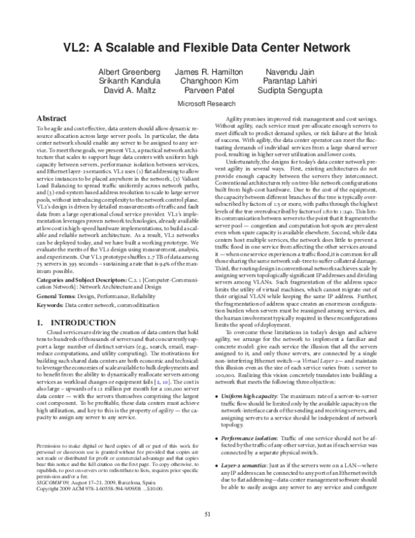
 Clara Kim