Robust tests for independence of two time series Pierre DUCHESNE∗† Roch ROY‡§ CRM-2751 August 2001 ∗ Service d’enseignement des méthodes quantitatives de gestion, École des Hautes Études Commerciales de Montréal This work was supported by grants from the Natural Science and Engineering Research Council of Canada and the Institut de Finance Mathématique de Montréal IFM2 . ‡ Département de mathématiques et statistique, Université de Montréal § This work was supported by grants from the Natural Science and Engineering Research Council of Canada, the Fonds FCAR (Government of Québec) and the Network of Centres of Excellence on the Mathematics of Information Technology and Complex Systems. † Abstract This paper aims at developing a robust and omnibus procedure for checking the independence of two time series. Li and Hui (1994) proposed a robustified version of Haugh’s (1976) classic portmanteau statistic which is based on a fixed number of lagged residual cross-correlations. In order to obtain a consistent test for independence against an alternative of serial crosscorrelation of an arbitrary form between the two series, Hong’s (1996a) introduced a class of statistics that take into account all possible lags. The test statistic is a weighted sum of residual cross-correlations and the weighting is determined by a kernel function. With the truncated uniform kernel, we retrieve a normalized version of Haugh’s statistic. However, several kernels lead to a greater power. Here, we introduce a robustified version of Hong’s statistic. We suppose that for each series, the true ARMA model is estimated by a n1/2 -consistent robust method and the robust cross-correlation is so obtained. Under the null hypothesis of independence, we show that the robust statistic asymptotically follows a N (0, 1) distribution. Using a result of Li and Hui, we also propose a robust procedure for checking independence at individual lags and a descriptive causality analysis in the Granger’s sense is discussed. The level and power of the robust version of Hong’s statistic are studied by simulation in finite samples. Finally, the proposed robust procedures are applied to a set of financial data. Key words and phrases: ARMA model; robust serial correlation; robust estimation; coherency; independence; causality. Mathematics subject classification codes (2000): primary 62M10; secondary 62F35. Résumé L’objectif premier de cet article est de développer une approche robuste afin de vérifier l’indépendance de deux séries chronologiques. Li et Hui (1994) ont proposé une version robuste de la statistique portmanteau de Haugh (1976) qui est basée sur les corrélations croisées résiduelles à un nombre fixé de délais. Afin d’obtenir un test convergent pour l’hypothèse d’indépendance par rapport à une alternative de corrélation sérielle croisée de forme quelconque, Hong (1996a) a introduit une classe de statistiques prenant en compte tous les délais. La statistique de test est une somme pondérée de toutes les corrélations croisées résiduelles, la pondération étant déterminée par une fonction de noyau. Avec le noyau uniforme tronqué, nous retrouvons une version normalisée de la statistique de Haugh. Cependant, plusieurs noyaux permettent d’obtenir une plus grande puissance. Dans ce travail, nous introduisons une version robuste de la statistique de Hong. Nous supposons que pour chaque série, le vrai modèle ARMA est estimé par une méthode robuste qui est n1/2 -convergente et les corrélations croisées résiduelles sont ainsi obtenues en utilisant une version robuste des corrélations croisées sérielles. Sous l’hypothèse nulle d’indépendance, nous montrons que la statistique robustifiée de Hong suit asymptotiquement une loi N (0, 1). De plus, en utilisant un résultat de Li et Hui, nous proposons une procédure robuste pour vérifier l’indépendance à chaque délai et une analyse descriptive de causalité au sens de Granger y est aussi décrite. Le niveau et la puissance de la statistique robustifiée de Hong sont étudiés par simulation en échantillons finis. Finalement, l’application de la méthodologie robuste proposée est illustrée à l’aide d’un jeu de données financières. 1. INTRODUCTION Several physical and economic phenomena can be described by time series; see among others Akaike and Kitagawa (1999) for physical applications and Judge, Hill, Griffiths, Lütkepohl and Lee (1985) for economic applications. When we have to deal with two time series, the question often arises of describing the interrelationships existing between them. In economics, for example, elucidation of causality relationships between time series may be very important in a prediction context. Before applying sophisticated methods for describing relationships between two time series, it is important to check whether they are independent (or serially uncorrelated in the non-Gaussian case) or not. If sufficiently powerful methods which are simple both to apply and to interpret were available for checking the independence of two time series, more sophisticated multivariate analyses as causality analysis might become redundant. Haugh’s (1976) paper is at our knowledge the first attempt at developing a procedure based on residual cross-correlations for checking the independence of two stationary ARMA series. It is a two-stage procedure. First, it involves fitting univariate models to each of the series and then, cross-correlating the two resulting residual series. Let rûv̂ (j) be the residual cross-correlation at lag j: Pn t=j+1 ût v̂t−j rûv̂ (j) = Pn , P ( t=1 û2t nt=1 v̂t2 )1/2 for |j| ≤ n − 1, where ût , v̂t , t = 1, . . . , n, are the two residual series and n is the length of each time series. The asymptotic distribution of a fixed number of residual cross-correlations is given by Haugh (1976). He considered a portmanteau statistic which is based on the first M residual cross-correlations, where M ≤ n − 1 is a fixed integer. More precisely, he introduced the statistic SM = n M X 2 rûv̂ (j). (1) j=−M Its asymptotic distribution is chi-square under the null hypothesis of independence, and the hypothesis is rejected for large values of the test statistic. Haugh’s procedure was extended in various directions. Koch and Yang (1986) introduced a modification of SM that allows for a potential pattern in the residual cross-correlation function. El Himdi and Roy (1997) proposed a version of SM for two stationary vector ARMA (VARMA) that was recently extended to partially non stationary (cointegrated) VARMA series by Pham, Roy and Cédras (2000). Hallin and Saidi (2001) have recently proposed a generalization of Koch and Yang procedure for VARMA series. In the application of Haugh’s procedure, a value of M must be chosen a priori. It cannot be too large in order that the asymptotic chi-square approximation be satisfactory. Since SM does not take into account the cross-correlations at lag j for j > M , it will not detect serial correlation at high lags and leads therefore to an inconsistent test procedure. The previous observation led Hong (1996a) to propose a generalization of Haugh’s statistic that takes into account all possible lags. Its test statistic is a weighted sum of residual cross-correlations of the form Qn = n Pn−1 j=1−n k 2 (j/m)r 2 (j) ûv̂ [2Vn (k)]1/2 − Mn (k) , (2) n−1 n−2 2 4 where Mn (k) = j=1−n (1 − |j|/n)k (j/m) and Vn (k) = j=2−n (1 − |j|/n)(1 − (|j| + 1)/n)k (j/m). The weighting depends on a kernel function k. With the truncated uniform kernel, Qn corresponds to a normalized version of Haugh’s statistic. However several kernels lead to a higher power than the truncated uniform kernel. Indeed, he shows that the so-called Daniell kernel maximizes the asymptotic power of his test in a certain class of smooth kernels and under some local alteratives. Also, Hong (1996a) avoids the ARMA modeling by fitting autoregressions of appropriate high orders. Hong’s techniques of proofs are different from those of Haugh, since he directly establishes the asymptotic distribution of Qn , without making use of the asymptotic distribution of a fixed length vector of residual cross-correlations. Under the null hypothesis, the test statistic Qn is asymptotically N (0, 1). The test is unilateral and rejects for the large values of Qn . P P 1 In practice, outliers in time series can create serious problems. They can occur for various reasons, namely because of measurement errors or equipment failure, etc. Haugh and Hong tests for independence are based on estimation methods that are sensitive to outliers. Furthermore, the usual cross-correlation function can be considerable affected by outliers. An interesting review of robust methods in time series is presented in Martin and Yohai (1985); see also Hampel, Ronchetti, Rousseeuw and Stahel (1986), Rousseeuw and Leroy (1987). Robust estimation methods in ARMA models are studied in Bustos and Yohai (1986), and a robustified autocovariance function is introduced. Robust estimation of VARMA models is considered in Ben, Martinez and Yohai (1999). Li and Hui (1994) proposed a robustified crosscorrelation function between two time series and employed it to develop a robust version of Haugh’s (1976) and McLeod’s (1979) tests for checking independence. They established the asymptotic normality of a fixed length vector of robust cross-correlations. Their robust portmanteau statistics also follow asymptotically a chi-square distribution. Another approach of the non-parametric type for checking the independence of two autoregressive time series based on autoregressive rank scores is studied by Hallin, Jurevcková, Picek and Zahaf (1999). The main objective of this paper is to develop a robust version of Hong’s statistic for checking the independence of two univariate stationary and invertible time series. The test statistic is based on the robust cross-correlation function introduced by Li and Hui (1994). We suppose that for each series, the true ARMA model is estimated by a n1/2 -consistent robust method and the residual robust cross-correlation function is so obtained. In the empirical part of the paper, we used the residual autocovariances estimators (RA estimators) introduced by Bustos and Yohai (1986). A robustified version of Qn is obtained by replacing in (2) the usual residual cross-correlation by the robust ones. As in El Himdi and Roy (1997), we also describe a robust procedure for checking independence at individual lags. It relies on a result of Li and Hui (1994). As emphasized by Box, Jenkins and Reinsel (1994) and others, it is important not only to look at the value of a global statistic but also to examine the values of the cross-correlations at individual lags. It may well happened that the procedure based on individual lags lead us to reject the null hypothesis whilst the global test does not reject. Also, if in a first step we reject with the global test, the tests at individual lags will identify the lags where there is a significant correlation. The organization of the paper is as follows. In Section 2, we introduce the notations, concepts and results employed thereafter. Invoking a general result in Li and Hui (1994), we describe in Section 3 a robust procedure for checking independence at individual lags and we present a robustified version of Haugh’s (1976) statistic. A descriptive approach for causality analysis in the Granger’s (1969) sense is also discussed. The main result of the paper is presented in Section 4. We establish under the null hypothesis the asymptotic normality of a robustified version of Hong’s statistic. The proof relies on a central limit theorem for martingale difference. It is long and involved and is deferred to an Appendix. In Section 5, we describe the results of a small Monte Carlo experiment conducted in order to analyze the level and power of the new statistics and to compare them to their non robust versions. The procedures introduced in the paper are applied to a set of financial data in Section 6 and we end with some concluding remarks. 2. PRELIMINARIES 2.1 Assumptions on the process Let {(Xt , Yt ), t ∈ Z} be a bivariate second-order stationary process. Without loss of generality, we can assume that {(Xt , Yt )} is centered at zero. We further suppose that {Xt } and {Yt } are of the ARMA type, that is φ1 (B)Xt = θ1 (B)ut , φ2 (B)Yt = θ2 (B)vt , h h where φh (B) = pi=0 φhi B i , θh (B) = qi=0 θhi B i , h = 1, 2, with θ10 = θ20 = 1 and B is the backward shift operator. We assume that the two processes are invertible. >From the stationarity and inversibility assumptions, it follows that the power series of the complex variable z given by {φh (z)}−1 θh (z) = ψh (z) = P∞ r −1 = π (z) = P∞ π z r converge for |z| ≤ 1 and that the coefficients {ψ } and h h,r r=0 ψh,r z and θh (z) r=0 h,r {πh,r } tends to zero exponentially. P P 2 The innovation processes {ut } and {vt } are strong white noise, that is the ut ’s and the vt ’s are two sequence of independent and identically distributed random variables with mean zero and variance σu2 and σv2 , respectively. It is also supposed that the fourth-order moment of ut and vt exist and that the probability distributions of ut and vt are symmetric with respect to zero. The symmetry assumption is frequent in the robustness context, see for example Denby and Martin (1979), Bustos, Fraiman and Yohai (1984) and Bustos and Yohai (1986). 2.2 Outliers in time series In time series, Fox (1972) introduced two types of outliers: the innovation outliers and the additive outliers. That terminology is frequently used in robustness studies, see for exemple Martin and Yohai (1985), Rousseeuw and Leroy (1987), Hampel, Ronchetti, Rousseeuw and Stahel (1986). Here, we briefly described these two types of outliers using a probability models as it is often done in distributional studies. a) Innovation outliers Suppose that {Xt } is an ARMA(p,q) process, as described in Section 2.1 and that the innovation process {ut } has an heavy tail distribution F with is not far from the Gaussian distribution, as for example a contaminated normal: F = (1 − ǫ)N (0, σ 2 ) + ǫN (0, τ 2 ), where ǫ > 0 is small, and τ ≥ σ. In this situation, the innovations ut are from a N (0, σ 2 ) with probability 1 − ǫ, or from a N (0, τ 2 ) with a larger variance with probability ǫ. The latter innovations are considered as outliers. The important point with innovation outliers is that the ARMA(p, q) model is still the exact model for the observations. However, if an outlier occurs at t0 , then ut0 will affect not only Xt0 , but many future observations Xt0 +1 , Xt0 +2 , and so on. After a while, the effect disappears. Bustos and Yohai (1986) give several results showing that innovation outliers do not affect too seriously the least square estimators of autoregressive and moving avevage parameters of an ARMA process. b) Additive outliers Suppose that the observations are obtained from the model Xt = X̃t + Vt , where {X̃t } is ARMA, that is φ1 (B)X̃t = θ1 (B)ut , the innovations ut are Gaussian with a common variance σ 2 , the Vt are iid random variables, independent of X̃t whose distribution is H = (1 − ǫ)δ0 + ǫG, where δ0 is the degenerated distribution at zero, and G is an arbitrary distribution. In that situation, the ARMA process itself is observed without error with probability 1−ǫ and there is a probability ǫ that the process ARMA plus an error of distribution G be observed. Least-square estimators and even M -estimators are quite sensible to additive outliers. Bustos and Yohai (1986) proposed alternative estimation methods with a good behavior in presence of such outliers. Since the ARMA(p, q) process {Xt }: φ(B)Xt = θ(B)ut is stationary and invertible, we can write Xt = φ−1 (B)θ(B)ut and ut = θ(B)−1 φ(B)Xt . To robustly estimate the ARMA parameters of the process {Xt }, Bustos and Yohai (1986) introduced the RA estimators (for Residual Autocovariances). These estimators are obtained by solving the equation system (3), which is similar to the one leading to the least squares estimators except that the usual sample innovation autocorrelation function γu (·) is replaced by P P a robustified version γu (·; η). Let φ−1 (z) = j≥0 sj z j and θ−1 (z) = j≥0 πj z j . The RA estimators are 3 obtained through the resolution of the following system: n−j−p−1 X h=0 n−j−p−1 X sj γu (h + j; η) = 0, j = 1, . . . , p; πj γu (h + j; η) = 0, j = 1, . . . , q; (3) h=0 n X ψ(ut /σu ) = 0. t=p+1 The robust autocorrelation γu (i; η) at lag i is defined by γu (i; η) = n−1 n X η(ut /σu , ut−i /σu ). (4) t=p+1+i We defined similarly γû (i; η) computed with the residual series. The scale parameter σu is estimated simultaneously from the observations using for example σ̂u = med(|ûp+1 |, . . . , |ûn |)/.6745. (5) Several choices for the function η are possible, as for example Mallows type or Hampel type functions: ηM (u, v) = ψ(u)ψ(v), Mallows, (6) ηH (u, v) = ψ(uv), Hampel, (7) where the function ψ is continuous and odd. Examples for the function ψ is the Huber family ψH (u; c) = sign(u) min(|u|, c); (8) and the bisquare family proposed by Beaton and Tukey (1974) which is defined by ψB (u; c) = ( u(1 − u2 /c2 )2 , if 0 ≤ |u| ≤ c, 0, otherwise. (9) Note that the function η(u, v) = uv leads to the usual autocorrelation function and the least-squares estimators are obtained by solving (3) with η(u, v) = uv and ψ(u) = u. Bustos and Yohai (1986) also introduced a class of truncated RA estimators (TRA) that behave well when additive outliers are present. An heuristic argument shows that these estimators are qualitatively robust when a moving average component is present in the ARMA model. The results presented in Section 3 are based on RA estimators although the main result of this paper described in Section 4 only required that the AR and MA estimators be n1/2 -consistent and robust. Other robust and consistent estimators could be used in conjunction with the robustified autocorrelation function γu (i; η). For example, GM estimators as well as RA and TRA estimators are n1/2 -consistent and robust. RA estimators with Mallows type function are particularly convenient to compute since an iterative scheme is possible. For rigor and completeness, we state explicitly the consistency condition in Assumption A. Assumption A: Let {Xt } and {Yt } be ARMA processes as described in Section 2.1. We suppose that the estimators of the parameters satisfy the following conditions: φhj − φ̂hj θhj − θ̂hj = Op (n−1/2 ), j = 1, . . . , ph ; h = 1, 2; = Op (n−1/2 ), j = 1, . . . , qh ; h = 1, 2; σu − σ̂u = Op (n−1/2 ); σv − σ̂v = Op (n−1/2 ). 4 With two time series, the cross-correlation function is often used to appreciate the existing dependency between the two processes. However, as the autocorrelation function, it is sensible to outliers. Li and Hui (1994) proposed the following robust cross-correlation function: γuv (j; η) = ( n−1 nt=j+1 η(ut /σu , vt−j /σv ), j ≥ 0, P n−1 nt=−j+1 η(ut+j /σu , vt /σv ), j < 0, P (10) where {ut } and {vt } are the two innovation processes, with variances σu2 and σv2 respectively. When η(u, v) = uv, we retrieve the usual sample cross-correlation function, and we write γuv (j; η) = ruv (j). Similarly, a robust residual cross-correlation function is obtained by replacing {ut } and {vt } by the residual series {ût } and {v̂t }. Li and Hui (1994) studied the asymptotic properties of a fixed length vector of robust residual cross-correlations. 3. TESTS BASED ON A SUBSET OF LAGS By making use of a general result of Li and Hui (1994) on the asymptotic distribution of a vector of robustified residual cross-correlations, we present in this section a robust procedure for testing the hypothesis of non correlation based on the robustified cross-correlations at a particular lag or at a finite number of lags. We also described a robustified version of the procedure for testing causality in the Granger (1969) sense discussed in El Himdi and Roy (1997). 3.1 Asymptotic distribution of robust cross-correlations The theorem of Li and Hui (1994) is based on RA-estimation of the ARMA parameters and is a direct generalization of a similar result in McLeod (1979) for least squares estimators. It also extends Haugh’s (1976) theorem. However, when going through the Taylor series expansions involved in Haugh’s proof (see also El Himdi and Roy, 1997), it is seen that Haugh’s approach remains valid for any n1/2 -consistent ARMA estimators. That remark leads us to Theorem 1 below which is slightly more general than the result of Li and Hui (1994) under the null hypothesis of non correlation between the two processes {Xt } and {Yt }. Let j1 , . . . , jm be a sequence of m distinct integers independent of n such that |ji | < n and let us consider the vector γ ηuv = (γuv (j1 ; η), . . . , . . . , γuv (jm ; η))′ . We have the following result. Theorem 1 Let {Xt } and {Yt } be two second-order stationary and invertible ARMA processes satisfying the assumptions of Section 2.1. Let {ût } and {v̂t } be the residual series resulting from n1/2 -consistent and √ √ robust estimation of the parameters. If the two processes are independent, then nγ ηûv̂ and nγ ηuv have the same asymptotic distribution Nm (0, aIm ), where a = E[η 2 (u1 /σu , v1 /σv )]. A similar result is given in Haugh (1976) for univariate time series and in El Himdi and Roy (1997) for multivariate time series, in the the particular case γ ηûv̂ = rûv̂ = (rûv̂ (j1 ), . . . , rûv̂ (jm ))′ and when the parameters are estimated by conditional least-squares. In the next two sections we apply Theorem 1. 3.2 Test based on the robust cross-correlation at a particular lag Suppose that we want to test in a robust manner that the two stationary and invertible ARMA processes {Xt } and {Yt } are uncorrelated, that is: H0 : ρuv (j) = 0, j ∈ Z, where ρuv (j) = corr(ut , vt−j ) is the population cross-correlation of lag j, between {ut } and {vt }. Theorem 1 allows us to construct a robust version of the tests given in El Himdi and Roy (1997). √ √ Under H0 , from Theorem 1, we have that nγûv̂ (ji ; η)/ a, i = 1, . . . , m, are asymptotically independent and identically distributed N (0, 1). For the alternative hypothesis, H1j : ρuv (j) 6= 0, 5 it is natural to consider the statistic 2 (j; η)/â, SR (j) = nγûv̂ and under H0 , SR (j) follows a χ21 distribution, where â is a consistent estimator of a. For example, when P P η is of the Mallows type, a consistent estimator for a is â = [n−1 nt=1 ψ 2 (ût /σ̂u )] × [n−1 nt=1 ψ 2 (v̂t /σ̂v )]. Thus, at the signification level α, H0 is rejected if SR (j) > χ21,1−α , where χ2m,p is the pth quantile of the χ2m distribution. Haugh (1976) used the statistics 2 S(j) = nrûv̂ (j) and noticed from a simulation study that the exact level can be much smaller than the asymptotic level, specially for high lags. He proposed the modified statistic S ∗ (j) = n S(j) n − |j| (11) which is much better approximated by the asymptotic distribution. For that reason, we also consider the robust modified statistic n ∗ SR (j) = SR (j) (12) n − |j| which is asymptotically equivalent to SR (j). In practice, we are often interested in considering simultaneously several lags, for example all lags such that |j| ≤ M , where M ≤ n − 1. Thus, the alternative hypothesis becomes in that situation (M ) H1 : There exists at least one j, |j| ≤ M, such that ρuv (j) 6= 0. A global test for H0 based on the statistics SR (j), |j| ≤ M , consists in rejecting H0 if for at least one lags j, SR (j) > χ21,1−α0 . To obtain a global level α, since the SR (j) are asymptotically independent, the marginal level α0 for each test must be α0 = 1 − (1 − α)1/(2M +1) . That method has the advantage of individual examination at each lag in a robust way. Portmanteau tests do not share that property. As in El Himdi and Roy (1997), that procedure can be represented graphically with the lag j on the horizontal axis and the value of SR (j) on the vertical axis. Such a graphical representation allows us to appreciate the dependency between the two residual series at several lags, and can be useful to explaining the reasons of the rejection of the null hypothesis. Such an analysis can also be useful in causality studies. 3.3 Links with causality In many economic studies, it is important to know the causality directions between two time series when they are correlated at possibly many lags. Following the lines of El Himdi and Roy (1997), the robust crosscorrelation analysis described in the previous section can be pursued further for that purpose. Granger causality is now a basic concept in econometrics and is discussed in most textbooks in the field. See for example Hamilton (1994, chap.11) and Lütkepohl (1993, chap.2). Suppose that {(Xt , Yt ), t ∈ Z} is stationary. In a general framework, the process {Xt } does not cause {Yt } in the Granger (1969) sense if the minimum mean square error linear predictor of Yt based on the information set {(Xs , Ys ), s ≤ t − 1} is the same as the one based on the information set {Ys , s ≤ t − 1}. In other words, {Xt } does not cause {Yt } is Yt cannot be predicted more efficiently if the information contained in Xs , s ≤ t − 1 is taken into account in addition to the information in Ys , s ≤ t − 1. A more formal definition of causality and characterizations of non causality in vector ARMA models in terms of AR and MA parameters are given in Boudjellaba, Dufour and Roy (1992, 1994). Suppose that {Xt } and {Yt } are individually described by univariate stationary and invertible ARMA models. Pierce and Haugh (1977) obtained a characterization of the absence of causality between {Xt } and {Yt } in function of the cross-correlation between the two innovation processes {ut } and {vt }. They showed that {Xt } does not cause {Yt } if and if ρuv (j) = 0, ∀j < 0 and {Yt } does not cause {Xt } if and only if ρuv (j) = 0, ∀j > 0. Therefore, the residual cross-correlation function can be useful for detecting causality directions between {Xt } and {Yt }. 6 Suppose that we want to test the null hypothesis of non correlation H0 against the alternative + H1M : ρuv (j) 6= 0, for at least one j such that 1 ≤ j ≤ M, where M > 0 is a fixed integer. It seems natural to consider residual cross-correlations at positive lags to + define the test statistic and if H0 is rejected in favor of H1M , we will conclude that {Yt } causes {Xt }. As in the previous section, we can do simultaneous tests at lags 1, 2, . . . , M or employ the portmanteau type statistic +∗ SRM = M X ∗ SR (j). (13) j=1 which asymptotically follows a χ2M distribution under H0 and the null hypothesis is rejected for large values + of SRM . Similarly, for the alternative hypothesis − H1M : ρuv (j) 6= 0, for at least one j such that − M ≤ j ≤ 1, the test statistic will be −∗ SRM = −1 X ∗ (j), SR (14) j=−M − which is also asymptotically χ2M under H0 . If H0 is rejected in favor of H1M , we will conclude that {Xt } causes {Yt }. The procedure described here for causality analysis does not constitute a statistical test in the usual sense, since the hypothesis of non causality which is the hypothesis of interest stands for the alternative hypothesis rather than the null. It is however a robustified version of a similar approach used, among others, by Pierce (1977) and Pierce and Haugh (1977) to identity causality directions between univariate time series. >From a statistical point of view, we would like to directly consider the null hypothesis H0+ : ρuv (j) 6= 0, j > 0, or H0− : ρuv (j) 6= 0, j < 0 versus the simple negation of H0+ or H0− . Li and Hui (1994) give the asymptotic distribution of the vector of residual robust cross-correlations γ̂ ηûv̂ in the general case of two correlated univariate ARMA series. The asymptotic covariance matrix is quite involved since it depends on the true models describing the two series, and except for the special case of only instantaneous causality between the two processes {Xt } and {Yt }, it seems difficult to exploit it in practice. 4. TEST PROCEDURE BASED ON ALL LAGS For the null hypothesis of non-correlation, Li and Hui (1994) proposed the following portmanteau test statistic M n X SRM = γ 2 (j; η), (15) â j=−M ûv̂ and its modified version ∗ SRM = M n n X γ 2 (j; η), â j=−M n − |j| ûv̂ (16) which are robust versions of Haugh’s (1976) statistics. Hong (1996a) introduces another generalization of Haugh’s statistic which leads to a class of consistent tests for serial cross-correlation of unknown form between the two time series. Here, we propose a robust version of Hong’s approach. It is based on a kernel-based statistic. The kernel k(·) satisfies the following assumption. Assumption B: The kernel k : R → [−1, 1] is a symmetric Rfunction, continuous at 0, having at most a ∞ finite number of discontinuity points and such that k(0) = 1, −∞ k 2 (z)dz < ∞. 7 The test statistic, denoted QRn is the following. QRn = nâ−1 Pn−1 2 (j/m)γ 2 (j; η) ûv̂ 1/2 [2Vn (k)] j=1−n k − Mn (k) , (17) n−1 n−2 2 4 where Mn (k) = j=1−n (1 − |j|/n)k (j/m) and Vn (k) = j=2−n (1 − |j|/n)(1 − (|j| + 1)/n)k (j/m). The smoothing parameter m is such that m = m(n) → ∞, but m(n)/n → 0 as n → ∞. Using the truncated uniform kernel, we retrieve a standardized version of Li and Hui’s (1994) statistic. Since R∞ 2 R∞ 4 limn→∞ m−1 Mn (k) = M (k) = −∞ k (z)dz < ∞, limn→∞ m−1 Vn (k) = V (k) = −∞ k (z)dz < ∞, Mn (k) and Vn (k) can be replaced by mM (k) and mV (k) respectively. The resulting statistic is P P Q∗Rn = na−1 Pn−1 2 (j/m)γ 2 (j; η) ûv̂ (2mV (k))1/2 j=1−n k − mM (k) , (18) which is asymptotically equivalent in distribution to QRn . These substitutions may lead to better finite sample approximations. Although QRn and Q∗Rn are defined in terms of cross-correlations, there are also coherency-based statistics (in the frequency domain). For a function g : [−π, π] → C, the normalized L2 norm is defined by ||g||2 = (2π)−1 Z π −π |g(ω)|2 dω, where | · | denotes the modulus of a complex number. The cross-spectral density (based on correlations) of two stationary processes {ut } and {vt } is given by fuv (ω) = ∞ X ρuv (j)e−ijω . j=∞ To simplify the discussion, assume that η is of the Mallows type. Then, a−1/2 γuv (j; η) can be interpreted as the sample cross-correlation at lag j of the winsorized series {ψ(ut /σu )} and {ψ(vt /σv )}. A kernel-based robust estimator is given by n−1 X fˆuv (ω) = a−1/2 k(j/m)γuv (j; η)e−ijω , j=−n+1 whose L2 norm is ||fˆuv ||2 = a−1 n−1 X 2 k 2 (j/m)γuv (j; η). j=−n+1 In our situation, {ut } and {vt } are two white noises and the complex coherency (at frequency ω) is given by fuv (ω) 2πfuv (ω) Cuv (ω) = = . 1/2 σ u σv {fuu (ω)fvv (ω)} Therefore, QRn and Q∗Rn are essentially standardized versions of the estimated coherency ||Ĉuv ||. Under the hypothesis that {ut } and {vt } are two mutually independent processes, the asymptotic distribution of QRn is the following. The symbol →L stands for convergence in law. Theorem 2 Suppose that the assumptions of Section 2.1, assumptions A and B are satisfied, and that m → ∞, m/n → 0. If the innovation processes {ut } and {vt }, are independent, then QRn →L N (0, 1). The proof which is an adaptation of the one of Hong (1996b) is long and technical and is presented in the Appendix. It is written in two parts. First, we establish the asymptotic normality of the pseudo-statistic Q̃Rn = na−1 Pn−1 2 (j/m)γ 2 (j; η) uv 1/2 (2Vn (k)) j=1−n k 8 − Mn (k) which is based on the two innovation processes {ut } and {vt }. To derive the asymptotic normality, we make use of Brown’s (1971) central limit theorem for martingale differences that can be found in many textbooks, namely in Taniguchi and Kakizawa (2000, Chap 1). A more general version for a triangular array of random variables is presented in Fuller (1996, Chap.6). The ARMA models describing the two series do not intervene in the first part since Q̃Rn is completely determined by the two innovation series {ut } and {vt }. The observed data and the estimated models are taken into account in the second part in which it is shown that Q̃Rn − QRn = op (1) and Theorem 1 follows. 5. SIMULATION RESULTS In the previous sections, we have introduced a robustified versions of Hong’s (1996a) statistics for checking lagged cross correlation between two ARMA time series which have interesting asymptotic properties. They also extend the robust portmanteau test proposed by Li and Hui (1994) which is a robustified version of Haugh’s (1976) classic statistic. >From a practical point of view, it is natural to inquire for the finite sample properties of these statistics, in particular their exact level and power whether or not there is outliers in the series under study. To partially answer that question, a Monte Carlo simulation was conducted. The ∗ and Q∗ were also included following modified versions of Haugh’s (1976) and Hong’s (1996a) statistics SM n in the experiment. M X n ∗ 2 SM = n rûv̂ (j), (19) (n − |j|) j=−M and Q∗n = n Pn−1 j=1−n k 2 (j/m)r 2 (j) ûv̂ [2mV (k)]1/2 − mM (k) . (20) 5.1 Description of the experiment To compare the omnibus robust statistics QRn , Q∗Rn to their non-robust counterparts Qn , Q∗n and also to ∗ , S ∗ the portmanteau statistics SM RM and SRM , independent realizations were generated from the following bivariate Gaussian VAR(1) process: Xt Yt ! = 0.5 0.0 0.0 0.5 ! Xt−1 Yt−1 ! 1.0 ρ ρ 1.0 ! + ut vt ! , t ∈ Z. (21) The covariance matrix of (ut , vt )′ is Σ= . (22) We considered ρ = 0.0 and ρ = 0.2. The first value corresponds to the situation where two independent AR(1) series are generated, and that situation allows us to study the level of the tests. In the second case, the two series are serially correlated and it allows us to compare the powers. For each realization, the portmanteau statistics were computed for M = 6, 12, 18. Each omnibus statistic was calculated for five different kernels that are described in Table 1. For each kernel, three different rates m given respectively by ⌊log(n)⌋, ⌊3.5n0.2 ⌋ and ⌊3n0.3 ⌋, were employed (⌊a⌋ denotes the integer part of a). These rates are discussed in Hong (1996c, p. 849). They lead respectively to the values m = 5, 8, 12 for the series length n = 100 and to m = 5, 9, 15 with n = 200. For more details on kernels, see Priestley (1981). To investigate the effect of outliers on the robust and non robust statistics, 10 000 realizations were generated from the Gaussian VAR(1) model (21) for each series length (n = 100, 200). For each realization, the following three scenarios were considered: Scenario 1 No contamination. Scenario 2 For n = 100, we subtracted systematically the value 10 to observations X26 and Y76 . Furthermore, for n = 200, we added the value 10 to X101 and Y151 , and we subtracted 10 to X176 . 9 Table 1: Kernels used in the calculation of the omnibus statistics Qn and QRn Truncated uniform kernel (TR): Bartlett (BAR): Daniell (DAN): Parzen (PAR): Bartlett-Priestley (BP):  1 if |u| ≤ 1, 0 elsewhere.  1 − |z| if |z| ≤ 1, k(z) = 0 elsewhere, sin(πz) k(z) =  πz , z ∈ R.  1 − 6(πz/6)2 + 6|πz/6|3 if |z| ≤ 3/π, 2(1 − |πz/6|)3 if 3/π ≤ |z| ≤ 6/π, k(z) =  0 elsewhere. p p sin(π 5/3z) 9 p − cos(π 5/3z)}, z ∈ R. k(z) = { 5π 2 z 2 π 5/3z k(z) = Scenario 3 In addition to scenario 2, for n = 100, we added to X51 and Y51 the value 10 and for n = 200, we subtracted to X126 and Y126 the value 10. Similar scenarios were employed in Li (1988) and Li and Hui (1994). The first scenario allows us to evaluate the performance of the statistics in the context of Gaussian VAR(1) series. The second scenario permits to evaluate the performance of the procedures when outliers occur at different points in time. Finally, in the third scenario, outliers occur in both series at the same points in time. For the robust statistics, we chose the Mallows type functions η defined by (6) and two ψ functions were employed: Huber (8) and bisquare (9) families. The tuning constant c in Huber family is 1.65 and in the bisquare family is 5.58 (Bustos and Yohai, 1986; Li and Hui, 1994). In the level study, 10 000 independent realizations were generated from model (21) and (22) with ρ = 0 for each value of n and the computations were made in the following way. All the computer programs were written in Fortran 77. (1) The Gaussian white noise (ut , vt )′ , t = 1, . . . , n, was generated using the subroutine G05EZF from the NAG library. (2) The initial values (X0 , Y0 )′ was generated from the exact bivariate Gaussian distribution using Ansley’s (1980) algorithm. The values (Xt , Yt )′ , t = 1, . . . , n, were obtained by solving the difference equation (21). (3) For each realization, univariate AR(1) models were separately estimated for each of the two series and the residual series {ût , t = 1, . . . , n} and {v̂t , t = 1, . . . , n} were obtained. The autoregressive parameter was estimated by least squares for the non robust statistics and the RA estimators was obtained from the iterative algorithm described in Bustos and Yohai (1986, Section 2) for the robust statistics. The Mallows type function η combined with Huber and bisquare functions ψ were used. The three scenarios for outliers were applied to each realization, which leads to 9 distinct estimates and therefore to 9 residual series {(ût , v̂t )′ , t = 1, 2, . . . , n}. ∗ , Q and Q∗ were computed from the least-squares residuals. (4) For each realization, the test statistic SM n n ∗ ∗ The value of SRM , SRM , QRn and QRn were obtained from the RA residuals. (5) Finally, for each series of length n and for each of the three nominal level (1, 5 and 10%), we obtained for each statistic, the number of rejections of the null hypothesis of non correlation between the two series, based on 10 000 realizations. The detailed results can be found in Duchesne (2000, Chap. 4) and a summary is presented in Table 2. The standard error of the number of rejections is 9.9 for the nominal level 1%, 21.8 for 5% and 30 for 10%. For example, at the nominal level 5%, the observed number of rejections is not significantly different from the expected number of rejections if it lies 10 in the interval [458, 542] at the significance level α = 0.05 and in the interval [444, 556] at the significance level α = 0.01. The power study was conducted in a similar way except that the correlation between ut and vt is ρ = 0.2. 5.2 Discussion of the level study For briefness, we just present the results for the nominal level 5% in Table 2. Further, since the results for Qn and QRn are similar to those for Q∗n and Q∗Rn respectively, only the results for the modified statistics are reported. Finally, since the numbers of rejections for the three kernels DAN, PAR and BP are similar, we just give the results for Daniell kernel which is optimal (greatest asymptotic power) kernel in a certain class of smooth kernels for Qn and Q∗n (Hong, 1996a, Section 4). Since the nominal level is 5%, all the numbers in Table 2 must be compared to 500. Under scenario 1 ∗ and S ∗ (no outlier), the levels of the portmanteau statistics SM RM are perfectly controled. Hong’s statistic Q∗n tends to overreject. When m = 5, its empirical level varies arround 7% with the BAR and DAN kernels, around 8% with the TR kernel and becomes closer to 5% as m increases. A similar trend was observed by Hong (1996a). The behavior of the robustified version Q∗Rn is similar to the one of Q∗n irrespective of the ψ function. ∗ and Q∗ are very Under scenarios 2 and 3, it is immediately seen that the unrobustified statistics SM n sensitive to outliers. In general, they dramatically underreject under scenario 2 and overreject under ∗ under scenarios 2 and 3, scenario 3. By opposition, the empirical level of the robustified statistics SM ∗ those of QRn with either Huber or the bisquare function ψ under scenario 2 and those of Q∗Rn with the bisquare function are similar to the ones observed under scenario 1 and are therefore reasonably close to 5 %. However, Q∗Rn with Huber function overrejects considerably under scenario 3, specially for small values of m with the three kernels and for all values of m with the kernel BAR. For that reason, the bisquare function seems preferable in practice. Globally as a function of m, the sizes of the robust statistics are improving as m increases. With respect to the series length, there is no obvious improvement when n goes from 100 to 200. 5.3 Discussion of the power study The number of rejections under the alternative hypothesis based on 10 000 realizations at the 5 % nominal level are reported in Table 3. The values on lines 1, 3 and 4 are based on the asymptotic critical values for scenarios 1, 2 and 3 respectively, whilst those in parentheses on line 2 correspond to scenario 1 and are based on the empirical critical values (ECV) obtained from the level study. In general, the powers obtained with the ECV are slightly smaller that those found with the ACV. It is not surprising since generally, the ∗ and Q∗ under scenarios 2 and 3 are of limited omnibus statistics Q∗n and Q∗Rn overreject. The power of SM n interest since these statistics are severally affected by outliers. The only scenario for which all the tests are comparable is scenario 1. First, it is very interesting to notice that the price to pay for using a robustified ∗ statistic rather than its unrobustified version is rather small. Indeed, the power of SRM is smaller than ∗ ∗ the one for SM but the difference is rather small and the same can be said of QRn in comparison with Q∗n . Since the behavior of Q∗n was already discussed in Hong (1996a), we focus on its robustified version Q∗Rn . Among the three kernels, the BAR kernel is in general more powerful than the DAN kernel and the latter is considerably more powerful than the TR kernel. This observation does not contradict the optimality result of Hong (1996a) which says that the DAN kernel is optimal in a certain class of smooth kernels since the BAR kernel is not in that class. The two ψ functions lead to similar powers in scenarios 1 and 2. In some cases with scenario 3, Huber functions leads to larger powers than the bisquare function. It is very likely related to the fact that the empirical levels are much larger than the nominal level. As a function of m, the power of Q∗Rn decreases considerably as m increases except with Huber function in scenario 3. As for Hong’s statistic Q∗n , the power of Q∗Rn increases very slightly when n goes from 100 to 200. Finally, among the three kernels, the TR kernel is the lest powerful but it is still more powerful ∗ . The empirical results presented here strongly than Li and Hui’s (1994) robust portmanteau statistics SM ∗ support the use of the new robust statistic QRn when additive outliers are suspected. Indeed, the loss of 11 Table 2: Number of rejections under the null hypothesis based on 10 000 realizations at the 5% nominal level. For each value of M or m, the three lines correspond to the three scenarios. Q∗Rn ∗ Qn Huber bisquare ∗ ∗ ∗ M SM SRM (H) SRM (b) m BAR DAN TR BAR DAN TR BAR DAN TR n = 100 6 460 469 478 5 753 657 835 776 657 842 769 664 828 36 463 462 175 119 121 737 625 828 748 649 850 2266 565 457 9480 8632 4754 1101 894 988 740 651 822 12 488 19 309 487 510 544 496 471 484 8 673 555 645 94 70 42 8581 6722 1876 670 650 960 542 552 715 651 636 750 674 670 661 544 556 545 647 658 654 18 469 10 58 478 534 576 484 476 471 12 575 432 57 31 6902 4073 566 586 767 425 427 539 470 500 535 580 590 565 438 437 436 477 461 474 509 21 7211 505 480 711 515 509 495 5 781 669 899 764 666 898 156 95 73 714 627 865 9997 9977 9101 1673 1365 1307 779 762 786 687 677 678 901 900 933 12 532 9 2186 499 496 619 504 500 499 9 678 590 737 677 585 62 45 28 636 564 9936 9740 5581 1348 1088 709 696 927 676 671 701 582 575 609 732 715 717 18 467 8 514 478 494 622 472 481 496 15 614 513 546 602 28 31 10 578 9498 9105 1437 1088 525 557 687 607 589 595 489 491 478 531 554 556 n = 200 6 12 473 17 407 501 482 827 Table 3: Number of rejections under the alternative hypothesis based on 10 000 realizations at the 5 % nominal level. For each value of M or m, the three lines correspond to the three scenarios. The values in parentheses represent the number of rejections based on the empirical critical values for scenario 1. ∗ SM M n = 100 6 1750 (1845) 98 5254 Q∗n DAN Q∗Rn Huber BAR DAN bisquare BAR DAN TR ∗ (H) SRM ∗ (b) SRM 1656 (1744) 1432 2240 1656 (1720) 1576 1584 5 4781 3802 2876 4571 (4033) (3400) (2153) (3890) 924 546 265 3962 9948 9787 7745 5970 3658 (3242) 3068 4930 2724 (2001) 2337 3543 4562 (3861) 4248 4446 3655 (3229) 3388 3528 2705 (1968) 2533 2576 8 3964 3020 2022 3814 (3520) (2871) (1668) (3421) 545 276 109 3213 9782 9153 4559 5092 m BAR TR TR 12 1349 (1382) 40 1246 1283 (1315) 1168 1708 1291 (1310) 1228 1257 2866 (2746) 2370 3976 1947 (1642) 1693 2530 3821 (3402) 3561 3693 2863 (2733) 2621 2708 1936 (1621) 1869 1891 18 1138 (1198) 23 308 1075 (1117) 1023 1459 1088 12 3288 2301 1411 3129 2129 (1112) (3067) (2488) (1460) (2918) (2325) 1024 298 112 39 2615 1773 1037 9241 7323 1623 4301 3021 1350 (1417) 1211 1808 3124 (2926) 2901 3003 2116 (2311) 2000 2019 1347 (1398) 1275 1318 n = 200 6 3780 (3748) 128 9612 3585 (3568) 2817 4883 3555 (3510) 3258 3351 5 7716 6858 5304 7489 (7145) (6394) (4103) (6919) 1422 890 377 6556 10000 10000 9943 8787 6639 (6157) 5627 8138 5082 (3945) 4137 6469 7492 (6902) 7095 7271 6623 (6137) 6185 6339 5077 (3933) 4663 4761 9 6769 5691 3872 6540 (6292) (5376) (3218) (6074) 746 430 120 5538 10000 9996 9072 8036 12 2687 (2583) 42 6304 2528 (2536) 2021 3558 2545 (2538) 2286 2419 5459 (5156) 4426 6999 3671 (3055) 3005 4873 6534 (6055) 6113 6281 5441 (5147) 4960 5134 3676 (3083) 3382 3514 18 2152 (2238) 16 2546 2058 (2122) 1650 2798 2051 15 5749 4410 2662 5539 4192 (2121) (5429) (4377) (2522) (5169) (4192) 1848 323 241 30 4500 3363 1921 9985 9938 5016 7027 5747 2516 (2428) 2034 3418 5499 (5178) 5071 5261 4177 (4202) 3811 3939 2510 (2422) 2296 2390 13 power in using Q∗Rn rather than its unrobustified version Q∗n is not important and we have also seen that Q∗n is very sensitive to outliers. If the outliers are at the same point in time, the bisquare function seems preferable to Huber function. 6. APPLICATION 6.1 The data We illustrate here the new robust tests for non correlation with a real data set coming from the financial literature. It was analyzed by Brockwell and Davis (1996, Chap. 7) who aimed at developing a stationary bivariate time series model. However, in practice, before deciding to build a multivariate model, a first important step is to check for cross-correlation between the series. If we conclude that they are indeed dependent, it is then appropriate to develop a multivariate model. 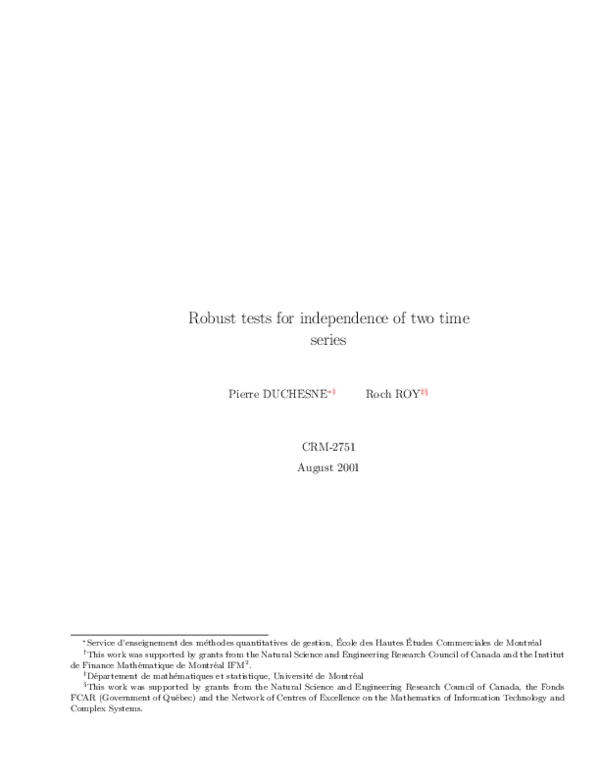Figure 1: Closing values of the Dow-Jones Index and of the Australian All-ordinaries index, for the period September 13, 1993 to August 26, 1994. Dow-Jones-All-ordinaries Indices DowJones AllOrdinaries Dow-Jones Index and Australian All-ordinaries Index 4000 3500 3000 2500 2000 0 50 100 150 200 250 Days The variables are the closing values of the Dow-Jones Index of stocks (Dt ) on the New York Stock Exchange and the closing values of the Australian All-ordinaries Index (At ) of Share Prices during 251 successive trading days from September 13, 1993 to August 26th, 1994. The two series are displayed in Figure 1. According to the efficient market hypothesis, these two series should behave individually as random walks with uncorrelated increments. In order to have stationary series, the data are transformed as percentage relative price changes: Xt Yt ! = 100(Dt − Dt−1 )/Dt−1 100(At − At−1 )/At−1 ! , t = 1, . . . , 250. The sample autocorrelations of each series indicate that both of them can be considered as white noise since all their autocorrelations are within or very close to the significant limits ±1.96n−1/2 (Brockwell and Davis, 1996, Example 7.1.1). The sample cross-correlations are also insignificant except at lag -1 where rXY (−1) = 0.46, which indicates that Xt−1 and Yt are dependent. 6.2 Correlation analysis The test procedures described in the previous sections can be directly applied to the two series since there is no significant serial autocorrelation. The values of the statistics S ∗ (j) defined by (11), |j| ≤ 12, are presented in Figure 2 (left part). With tests at individually lags, we strongly reject the hypothesis of non-correlation at lag j = −1. We also reject with simultaneous tests at lags −6, . . . , +6 and even at lags ∗ (j), |j| ≤ 12, are also −12, . . . , +12 at the global level α = 0.05. The values of the robust statistics SR 14 Table 4: Values of the statistics Q∗n and Q∗Rn for the real data and for the data contaminated by two outliers. Real data Contaminated data ∗ ∗ M Qn Q∗n QRn Q∗Rn 5 16.75 11.25 0.45 10.18 9 13.58 9.05 0.37 8.18 16 10.43 7.03 -0.13 6.27 shown in the right part of Figure 2. Again, the non-correlation hypothesis is rejected by the test at the individual lag j = −1 and by the simultaneous tests at the global level α = 0.05. 25 20 15 0 0 5 5 10 VALUE OF THE TEST STATISTIC 40 35 30 25 20 15 10 VALUE OF THE TEST STATISTIC 45 30 50 55 35 ∗ (j) (right part) for different lags j with the Figure 2: Values of the statistics S ∗ (j) (left part) and of SR real data. The horizontal dotted line represents the marginal critical value at the level α = 0.05. The dash lines give the critical values at the global level α = 0.05, for simultaneous tests at lags j = −6, . . . , 6 and j = −12, . . . , 12. -12 -10 -8 -6 -4 -2 0 2 4 6 8 10 12 -12 LAG -10 -8 -6 -4 -2 0 2 4 6 8 10 12 LAG In order to take into account all possible lags, Hong’s test Q∗n and its robustified version Q∗Rn where carried out. The statistic Q∗Rn was calculated with the Daniell kernel and for the three values 5, 9, 16 for m that correspond to the three rates employed in Section 5. The scale parameters σX and σY in (4) were estimated with the median estimator defined by (5). The values of the statistics are reported in Table 4. At the 1% significance level, these values must be compared to the 99th quantile of the N (0, 1) distribution and again, the hypothesis of non correlation is rejected. Since there is no apparent outliers in the two series under study, we have replaced X219 by -5.5 and X205 by +5.5 which gives rise to two additive outliers in the Dow-Jones series. The contaminated series {Xt } and the series {Yt } are shown in Figure 3. Their behavior is comparable to the one of many financial time series. The new series {Xt } can still be considered as a white noise and the cross-correlation at lag j = −1 is now 0.14 rather that 0.46. For these new series, we have redone the correlation analysis. With the non robust procedure, cross-correlation is detected by the tests at individual lags as shown in Figure 4 (left part). However, no significant correlation is detected by the simultaneous tests at lags j = −12, . . . , 12 and j = −6, . . . , 6 as well as with Hong’s statistic whose values are reported in Table 4. With the robust ∗ (j) and in Table 4 for the statistics procedure as illustrated in Figure 2 (right part) for the statistic SR ∗ QRn , the hypothesis of non correlation is strongly rejected once again. 6.3 A descriptive causality analysis Once the hypothesis H0 of non correlation between the two series is rejected, it is natural to inquire into the directions of causality between the two variables, specially in economic studies. In Section 3.3, we have seen that {Xt } does not cause {Yt } if and only if ρuv (j) = 0, ∀j < 0, and {Yt } does not cause {Xt } is 15 Figure 3: The two variables Xt and Yt with two outliers. Percentage Relative Price for Dow-Jones and Australian All-ordinaries Index Percentage Relative Price for Dow-Jones-All-ordinaries Indices with outliers 6 DowJones AllOrdinaries 4 2 0 -2 -4 -6 0 50 100 150 200 250 Days +∗ −∗ +∗ −∗ Table 5: p-values of the non-robust tests SM , SM and of the robust tests SRM and SRM for the real data and for the contaminated data. Real data Contaminated data + − + − + − + − M SM SM SRM SRM SM SM SRM SRM 1 0.40 0+ 0.22 0+ 0.39 0.03 0.20 0+ + + 2 0.51 0 0.34 0 0.47 0.09 0.30 0+ 3 0.50 0+ 0.39 0+ 0.68 0.19 0.39 0+ + + 6 0.80 0 0.67 0 0.76 0.16 0.72 0+ + + 12 0.79 0 0.55 0 0.89 0.23 0.66 0+ Note: 0+ denotes a positive number smaller than 10−5 . and only if ρuv (j) = 0, ∀j > 0, where {ut } and {vt } are the two corresponding innovation processes. In the first part of the correlation analysis of the previous section, we have tested H0 with statistics based on individual lags and it is immediately seen from Figure 2 that ρuv (−1) is significantly different from zero and all the other lags, the values of the test statistics are either smaller than the 5% critical value or very close of it. Figure 2 leads us to think that the Dow-Jones Index influenced the Australian Index and that the Australian Index does not influence the Dow-Jones. Given the relative size of the two economies, it is not a surprising conclusion. P +∗ ∗ In order to simultaneously consider many lags, we can employ the statistic SM = M j=1 S (j) or P −∗ + +∗ ∗ 2 SM = −1 j=−M S (j) which are asymptotically χM under H0 . For H0 against H1M , the p-values of SM for − −∗ various values of M are presented in Table 5. For H0 against H1M , similar results are given for SM . Thus, − + for all the values of M considered, H0 is rejected against H1M and not rejected against H1M . These tests +∗ −∗ confirms the conclusion deduced from the graphical analysis. The robust statistics SRM and SRM defined by (13) and (14) respectively were also employed for these data and the conclusion are the same. The causality analysis was redone with the contaminated data and the resulting p-values are shown + − in Table 5. With the non robust statistics, H0 is not rejected against H1M as before. Against H1M , H0 is barely rejected at the 5% level at M = 1 and is not rejected at the other values of M . It is therefore difficult to conclude in that case. However, with the robust statistics, we retrieve the conclusions obtained with the true data. 16 25 20 15 0 0 1 5 10 VALUE OF THE TEST STATISTIC 8 7 6 5 4 3 2 VALUE OF THE TEST STATISTIC 30 9 35 10 ∗ (j) (right part) for different lags j with Figure 4: Values of the statistics S ∗ (j) (left part) and of SR the contaminated data. The horizontal dotted line represents the marginal critical value at the level α = 0.05. The dash lines give the critical values at the global level α = 0.05, for simultaneous tests at lags j = −6, . . . , 6 and j = −12, . . . , 12. -12 -10 -8 -6 -4 -2 0 2 4 6 8 10 12 -12 -10 -8 -6 LAG -4 -2 0 2 4 6 8 10 12 LAG CONCLUSION We proposed in this paper a robust version of Hong’s statistic for checking the independence of two univariate stationary and invertible ARMA time series. The robustified test statistic is obtained by replacing the usual residual cross-correlations by the robust ones, as introduced by Li and Hui (1994). We established under the null hypothesis the asymptotic normality of the new robustified test statistic. We described a robust procedure for checking independence at individual lags, following an approach similar to El Himdi and Roy (1997). A descriptive approach for causality analysis in the Granger’s (1969) sense is also discussed. In a Monte Carlo experiment, we analyzed the level and power of the new statistics and we compare them to their non robust versions. We used the residual robust autocovariance estimators introduced by Bustos and Yohai (1986) to perform the robust estimation of the ARMA parameters. However, any n1/2 -consistent robust method in conjunction with the use of the residual robust cross-correlation function are sufficient for the asymptotic normality. The empirical results presented show that Hong’s test is very sensitive to outliers and support the use of the new robust statistic when additive outliers are suspected. Our empirical results seem to indicate that the loss of power in using the new test rather than its unrobustified version is not important. APPENDIX Here is the proof of Theorem 2. In the following, ∆ represents a finite positive constant that can differ from one place to another. Let kjm = k(j/m) and ηt,s = η(ut /σu , vs /σv ). First, we establish the following result: Part 1 Under the assumptions of Theorem 2, Q̃Rn →L N (0, 1). 2 2 Proof: Let Tn = na−1 n−1 j=−n+1 kjm γuv (j; η). We treat separately the two cases j ≥ 0 and j < 0 and in 2 both of them, we decompose γuv (j; η) in two terms: For j ≥ 0, we show that P 2 γuv (j; η) = n−2 n X 2 ηt,t−j + 2n−2 n X 2 ηt−j,t + 2n−2 n X t−1 X ηt,t−j ηs,s−j , n X t−1 X ηt−j,t ηs−j,s . t=j+2 s=j+1 t=j+1 and if j < 0, we have that 2 γuv (j; η) = n−2 t=j+2 s=j+1 t=j+1 17 We can write Tn in the following manner: Tn = na −1 n−1 X 2 2 kjm γuv (j; η) + na −1 n−1 X 2 2 kjm γuv (−j; η), j=0 j=0 = (H1n + H2n ) + (W1n + W2n ) = Hn + Wn , where n n X X X X 1 n−1 1 n−1 2 2 2 2 ), H2n = ), ηt,t−j ηt−j,t ( ( kjm kjm na j=0 na t=j+1 t=j+1 j=1 H1n = t−1 t−1 n n X X X X X X 2 n−2 2 n−2 2 2 ηt,t−j ηs,s−j ), W2n = ηt−j,t ηs−j,s ). k ( k ( na j=0 jm t=j+2 s=j+1 na j=1 jm t=j+2 s=j+1 W1n = 2 ), ∀s, t, we have that Let us evaluate E(Hn ). Since a = E(ηs,t n X X X 1 n−1 1 n−1 2 2 2 E(H1n ) = E(ηt,t−j )] = kjm [ kjm (n − j)a. an j=0 an t=j+1 j=0 2 Also, E(H2n ) = n−1 j=1 kjm (1−j/n), and it follows that E(Hn ) = Mn (k). We further show that E(Wn ) = 0. Note that for s < t, E(ηt−j,t ηs−j,s ) = 0 and E(ηt,t−j ηs,s−j ) = 0, since η(·, ·) is an odd function in each variable, that {ut } and {vt } are independent strong white noises with symmetric distributions. Then, we can affirm that P n−1 X 2 2 γuv kjm (j; η) = Op (m/n). j=−n+1 To establish Part 1, we will show the following two results: Hn − Mn (k) [2Vn (k)]1/2 Wn (ii) [2Vn (k)]1/2 (i) →P 0, →L N (0, 1). We begin with (i). The result is established if we prove the next proposition: Proposition 1 E[Hjn − E(Hjn )]2 = O(m2 /n), j = 1, 2. Proof: We show the result for j = 1. The case j = 2 is similarly obtained. We note that H1n − E(H1n ) = n−1 X 2 kjm [n−1 j=0 n X 2 (ηt,t−j /a − 1)] n X 2 /a − 1)]2 )1/2 }2 . (ηt,t−j t=j+1 and using Minkovski’s inequality, we have that n−1 X E[H1n − E(H1n )]2 ≤ { 2 (E[n−1 kjm t=j+1 j=0 Proposition 1 is verified if we show that E[n−1 n X t=j+1 2 (ηt,t−j /a − 1)]2 = O(n−1 ), uniformly in j. 18 But we have [n−1 n X t=j+1 2 /a − 1)]2 = n−2 (ηt,t−j n X t=j+1 2 /a − 1)2 + (ηt,t−j n X 2n−2 t−1 X t=j+2 s=j+1 and thus E[n−1 n X t=j+1 2 (ηt,t−j /a − 1)]2 = 2 2 (ηt,t−j /a − 1)(ηs,s−j /a − 1), n−j 2 E[η1,1 /a − 1]2 = O(n−1 ). n2 Since E[(Hn −Mn (k))/(2Vn (k))1/2 ] = 0 and var[(Hn −Mn (k))/(2Vn (k))1/2 ] = var(Hn )/(2Vn (k)) = O(m/n), and since by hypothesis m/n → 0, we have shown (i). Pn P Pt−1 We now show (ii). We do a change in the indices of summation noting that n−2 t=j+2 j=1 s=j+1 = Pn Pt−1 Ps−1 Pn−2 Pn Pt−1 Pn Pt−1 Ps−1 t=3 t=j+2 t=2 s=2 s=1 j=1 . Also j=0 s=j+1 = j=0 . We can write Wn = 2a−1 η1,1 (n−1 n X ηt,t ) + Wn′ , t=2 where Wn′ is defined by Wn′ = n−1 = n−1 t−1 s−1 n X X X 2 2a−1 kjm ηt,t−j ηs,s−j + n−1 t−1 s−1 n X X X 2 2a−1 kjm ηt−j,t ηs−j,s , t=3 s=2 j=1 t=3 s=2 j=0 n X (W1nt + W2nt ) = n−1 t=3 n X Wnt , t=3 with the following definitions for W1nt and W2nt : W1nt = t−1 s−1 X X 2 ηt,t−j ηs,s−j , 2a−1 kjm s=2 j=0 W2nt = t−1 s−1 X X 2 2a−1 kjm ηt−j,t ηs−j,s . s=2 j=1 We remark that 2a−1 η1,1 (n−1 nt=2 ηt,t ) = op (1) and that term can be neglected in the sequel. We note that (Wnt , Ft ) is a martingale difference sequence, where Ft = σ[(us , vs ), s ≤ t]. Indeed, we verify that E(W1nt |Ft−1 ) = 0 since E[ηt,t−j ηs,s−j |Ft−1 ] = 0. We proceed in a similar way forpW2nt . To prove (ii), we use a theorem of Brown (1971), and in our context that theorem says that Wn / var(Wn ) →L N (0, 1) if we verify the following two conditions: P (A1) (A2) n n−2 X 2 χ(|Wnt | > ǫn[var(Wn )]1/2 )] → 0, ∀ǫ > 0, E[Wnt var(Wn ) t=3 n n−2 X Ẅ 2 →P 1, var(Wn ) t=3 nt 2 = E(W 2 |F where Ẅnt nt t−1 ) and χ(A) denotes the indicator function of the set A. We begin with (A1). It is sufficient to verify the following Liapounov’s condition: σ −4 (n)n−4 n X t=3 4 E(Wnt ) → 0, where σ 2 (n) = 2Vn (k). The following proposition gives the variance of Wn′ . 19 Proposition 2 var(Wn′ ) = σ 2 (n). Proof: 2 ) = E(W 2 ) + E(W 2 ), since E(W E(Wnt 1nt W2nt ) = 0, this can be deduced from the fact that 1nt 2nt E[ηt,t−j1 ηs1 ,s1 −j1 ηt−j2 ,t ηs2 −j2 ,s2 ] = 0, t > s1 , t > s2 . 2 , we obtain Developing W1nt 2 W1nt = 4a−2 t−1 s−1 X X ( 2 kjm ηt,t−j ηs,s−j )2 + s=2 j=0 −2 8a t−1 sX 2 −1 1 −1 sX 1 −1 sX X kj21 m kj22 m ηt,t−j1 ηs1 ,s1 −j1 ηt,t−j2 ηs2 ,s2 −j2 s1 =3 s2 =2 j1 =0 j2 =0 2 ) = 4a−2 and E(W1nt Pt−1 Ps−1 2 2 j=0 kjm ηt,t−j ηs,s−j ) ], s=2 E[( since E(ηt,t−j1 ηs1 ,s1 −j1 ηt,t−j2 ηs2 ,s2 −j2 ) = 0, s2 < s1 , s1 < t, s2 < t. 2 ), we have that Developing the square sum in E(W1nt s−1 X ( 2 kjm ηt,t−j ηs,s−j )2 = s−1 X 4 2 2 kjm ηt,t−j ηs,s−j +2 2 )=4 and then E(W1nt Pt−1 Ps−1 s=2 kj21 m kj22 m ηt,t−j1 ηs,s−j1 ηt,t−j2 ηs,s−j2 , j1 =1 j2 =0 j=0 j=0 s−1 1 −1 X jX 4 j=0 kjm , since E(ηt,t−j1 ηs,s−j1 ηt,t−j2 ηs,s−j2 ) = 0, t > s, j1 > j2 , t−1 s−1 4 2 2 2 ) = 4 and also E(ηt,t−j ηs,s−j ) = a2 . We show in a similar way that E(W2nt s=2 j=1 kjm and it implies P P s−1 t−1 4 2 that E(Wnt ) = 4 s=2 |j|=0 kjm . By calculations analogous to those in Hong (1996b), we show that P var(Wn′ ) = n−2 n X 2 ) = 4n−2 E(Wnt = 2 |j|=0 4 , kjm t=3 s=2 |j|=0 t=3 n−2 X t−1 s−1 n X X X P 4 (1 − (|j| + 1)/n)(1 − |j|/n)kjm = 2Vn (k). and the proof of Proposition 2 is completed. Writing W1nt and W2nt in the following manner: W1nt = 2a−1 W2nt = 2a−1 t−1 X s=2 t−1 X (1) Gt,s , (2) Gt,s , s=2 (1) where Gt,s = Ps−1 2 j=0 kjm ηt,t−j ηs,s−j , (2) t > s and Gt,s = Ps−1 (i)4 Lemma 1 E(Gts ) = O(m2 ), t > s, i = 1, 2. 20 2 j=1 kjm ηt−j,t ηs−j,s , t > s, we prove the next lemma. Proof: (1) (1)4 We present the proof for Gts , the other case being similar. We first develop Gts and evaluating the expectation, we obtain that (1)4 E(Gts ) s−1 X = 8 kjm E[(ηt,t−j ηs,s−j )4 ] + j=0 kj41 m kj42 m E[(ηt,t−j1 ηs,s−j1 )2 (ηt,t−j2 ηs,s−j2 )2 ], X ∆ j1 <j2 ≤ ∆( s−1 X 8 + kjm X j1 <j2 j=0 kj41 m kj42 m ) ≤ ∆( n−1 X 4 2 ) = O(m2 ). kjm j=0 (1)4 In the first equality, the other terms in the development of Gts have 0 expectation; this property is obtained by conditioning on the {ut } process. The second inequality follows from the fact that the moments in that expression are finite. With the preceding lemma, we can show the following proposition. 4 ) = O(t2 m2 ), i = 1, 2. Proposition 3 E(Wint Proof: 4 We present the proof for W1nt , the one for W2nt being similar. Developing W1nt and evaluating the expectation, we obtain that 4 ) = 16a−4 { E(W1nt t−1 X (1)4 E(Gts ) + ∆ X (1)2 (1)2 E(Gts1 Gts2 )}. s1 <s2 s=2 Since by conditioning on the {vt } process, it is easily seen that the other terms have 0 expectation. Then we obtain 4 E(W1nt ) ≤ ∆ t−1 t−1 X X s1 =2 s2 =2 ≤ ∆{ t−1 X s=2 (1)2 (1)2 E(Gts1 Gts2 ) ≤ ∆ t−1 t−1 X X (1)4 (1)4 [E(Gts1 )E(Gts2 )]1/2 , s1 =2 s2 =2 (1)4 [E(Gts )]1/2 }2 = O(t2 m2 ). This completes the proof of the proposition and condition (A1) follows since σ −4 (n)n−4 n X 4 ) = O(n−1 ). E(Wnt t=3 2 = Ẅ 2 + Ẅ 2 , where we let It remains to establish the validity of condition (A2). First note that Ẅnt 1nt 2nt P P 2 = 4a−2 E[( t−1 G(1) )2 |F 2 = 4a−2 E[( t−1 G(2) )2 |F Ẅ1nt ] and Ẅ ]. Again, we give the details for t−1 t−1 2nt s=2 ts s=2 ts 2 ; the development for Ẅ 2 is similar. First, Ẅ 2 can be developed in the following way: Ẅ1nt 2nt 1nt 2 2 ) + 4a−2 C1nt + 4a−2 C2nt + 4a−2 C3nt , = E(Ẅ1nt Ẅ1nt where 2 E(Ẅ1nt ) = 4 t−1 s−1 X X 4 kjm , C1nt = s=2 j=0 C2nt = 2 s=2 j=0 t−1 s−1 1 −1 X jX X s=2 j1 =1 j2 =0 C3nt = 2 t−1 sX 1 −1 X s1 =3 s2 =2 t−1 s−1 X X 4 2 2 kjm E[ηs,s−j ηt,t−j − a2 |Ft−1 ], kj21 m kj22 m E[ηt,t−j1 ηt,t−j2 ηs,s−j1 ηs,s−j2 |Ft−1 ], (1) (1) E[Gts1 Gts2 |Ft−1 ]. The following lemma will be useful in the sequel, and is a generalization of a result of Hong (p.4, 1996b). 21 Lemma 2 For t2 > s2 , t1 > s1 , (1) (1) (1) (1) |E[E(Gt1 s1 Gt1 s2 |Ft1 −1 )E(Gt2 s1 Gt2 s2 |Ft2 −1 )]| ≤ ( 2 2 ∆m2 (m−1 n−1 j=0 kjm ) , if t1 = t2 , P 2 2 ∆m(m−1 n−1 if t1 < t2 . j=0 kjm ) , P Proof: To prove the result, we proceed as in Hong (p.4, 1996b) using the Assumptions on the function η and the fact that {ut } and {vt } are independent with a symmetric distribution. The details are omitted. The terms C1nt and C2nt have the following properties. 2 ) = O(t2 m + tm2 ), E(C 2 ) = O(tm3 ). Proposition 4 E(C1nt 2nt Proof: P We first establish the result for C1nt . Let us write C1nt = t−1 s=2 C1nst , where C1nst = s−1 X j=0 2 2 − a2 |Ft−1 ]. ηt,t−j E[ηs,s−j Developing the square sum, we obtain 2 C1nt = t−1 X 2 C1nst +2 s=2 t−1 sX 1 −1 X C1ns1 t C1ns2 t s1 =3 s2 =2 2 2 and we study the two parts separately. For the first term, we easily show that E( t−1 s=2 C1nst ) = O(tm ). 2 )= The study of the second term allows us to conclude that it is of order O(t2 m) and it follows that E(C1nt 2 2 O(t m + tm ). Now let us study C2nt . Making changes in the indices of summation, C2nt can be written in the following manner: P C2nt = 2 t−2 X t−2 X t−1 X j1 +1 j2 =j1 +1 s=j2 +1 = 2 t−2 X kj21 m kj22 m E[ηt,t−j1 ηt,t−j2 ηs,s−j1 ηs,s−j2 |Ft−1 ], kj21 m C2nj1 t , j1 +1 where C2nj1 t = t−2 X t−1 X l1 =j1 +1 s=l1 +1 kl21 m E[ηt,t−j1 ηt,t−j2 ηs,s−j1 ηs,s−j2 |Ft−1 ]. 2 , we obtain Developing C2nt 2 C2nt =4 t−2 X 2 kj41 m C2nj 1t j1 =1 +8 t−2 jX 1 −1 X kj21 m kj22 m C2nj1 t C2nj2 t , j1 =2 j2 =1 4 2 and we analyze the two terms separately. The study of the first term allows us to show that E( t−2 j1 =1 kj1 m C2nj1 t ) = 2 ) = O(m3 t). We can O(m3 t) and the expectation of the second term is zero. Therefore, we have E(C2nt Pn 2 −2 −2 now establish (A2). We want to show that m var(n t=3 Ẅ1nt ) → 0, and similarly for Ẅ2nt . Since P m−2 var(n−2 n X 2 Ẅ1nt ) = m−2 E{(n−2 t=3 = m−2 E[(n−2 n X [Ẅ1nt − E(Ẅ1nt )])2 }, t=3 n 3 X X i=1 t=3 22 4a−2 Cint )2 ], it is sufficient to show that m−2 E[(n−2 n X t=3 for i = 1, 2, 3. Using Proposition 4, we have that m−2 E[n−2 n X t=3 Cint )2 ] → 0, n X C1nt ]2 ≤ m−2 n−4 { t=3 2 E(C1nt )1/2 }2 = O(m−1 + n−1 ). Also, we obtain that m−2 E[n−2 n X t=3 C2nt ]2 ≤ m−2 n−4 { n X t=3 2 E(C2nt )1/2 }2 = O(m/n) and finally, m−2 E[n−2 n X C3nt ]2 = m−2 n−4 t=3 n X 2 E(C3nt ) + 2m−2 n−4 n tX 2 −1 X E(C3nt1 C3nt2 ). t2 =3 t1 =2 t=3 But we verify that E(C3nt1 C3nt2 ) = 4 tX 2 −2 1 −1 sX s2 =3 s1 =2 E[E(Gt1 s1 Gt1 s2 |Ft1 −1 )E(Gt2 s1 Gt2 s2 |Ft2 −1 )]. n 2 ) ≤ ∆m2 t2 and E(C 2 −2 −2 2 Thus E(C3nt 3nt1 C3nt2 ) ≤ ∆mt1 by Lemma 2. Therefore, m E[n t=3 C3nt ] = O(n−1 + m−1 ), since m/n → 0, m → ∞, and condition (A2) is valid. This completes the proof of step 1. P Part 2 We have to prove that Q̃Rn − QRn = op (1). Then we have to show that n−1 X j=1−n √ 2 2 2 (j; η) − γûv̂ (j; η)] = op ( m/n), [γuv kjm since Vn (k) = O(m). 2 (j; η) − γ 2 (j; η) = [γ (j; η) − γ (j; η)]2 + Using the identity a2 − b2 = (a − b)2 + 2b(a − b), we can write γûv̂ uv ûv̂ uv 2γuv (j; η)[γûv̂ (j; η) − γuv (j; η)] and it is enough to show the two following results: n−1 X (B1) j=1−n n−1 X (B2) j=1−n √ 2 kjm [γûv̂ (j; η) − γuv (j; η)]2 = op ( m/n), √ 2 kjm γuv (j; η)[γûv̂ (j; η) − γuv (j; η)] = op ( m/n). We write n−1 j≥0 and we present the details for j ≥ 0, the other case being similar. j<0 + j=1−n = In the sequel, we make use of Taylor expansions of the residuals ût and v̂t . Such expansions are given in Box and Pierce (1970) for univariate ARMA processes and in Hosking (1980) for the multivariate case. P P P Proposition 5 ût = ut + v̂t = vt + p1 X ∞ X r=1 i=0 p2 X ∞ X r=1 i=0 Π1i (φ̂1r − φ1r )Xt−r−i − Π2i (φ̂2r − φ2r )Yt−r−i − 23 q1 X ∞ X r=1 i=0 q2 X ∞ X r=1 i=0 Π1i (θ̂1r − θ1r )ut−r−i + λunt , Π2i (θ̂2r − θ2r )vt−r−i + λvnt . For a proof, see for example Lemma 1 of Hosking (1980). Remark that Hosking (1980) writes λunt = Op (n−1 ). Here, we prefer to retain the eventual dependence with respect to t of the remainders and we P write λunt and λvnt . However, from Hosking’s proof, we can conclude that n−1 nt=1 λunt = Op (n−1 ) and P P P n−1 nt=1 λvnt = Op (n−1 ). We also have that n−1 nt=1 λ2unt = Op (n−2 ) and n−1 nt=1 λ2vnt = Op (n−2 ). The following lemma which gives us results on the orders in probability of the differences δut = ut − ût and δvt = vt − v̂t directly follows from Proposition 5. Lemma 3 n−1 Pn 2 t=1 δut = Op (n−1 ), n−1 Pn 2 t=1 δvt = Op (n−1 ). To show (B1) and (B2) we need results on γûv̂ (j; η) − γuv (j; η) and a Taylor series expansion of the η function will be used. Proposition 6 Let η1 (u, v) = ∂η(u, v)/∂u and η2 (u, v) = ∂η(u, v)/∂v. Then we have γûv̂ (j; η) − γuv (j; η) = −n−1 σu−1 n−1 σv−1 n X t=j+1 n X η1 (ut /σu , vt−j /σv )δut − η2 (ut /σu , vt−j /σv )δv,t−j + Rnt , t=j+1 where the remainder Rnt is such that Rnt = Op (n−1 ). Proof: This result is established in Li and Hui (p. 106, 1994) for the autoregressive case and can be easily generalized to the ARMA case. It is sufficient to write a Taylor expansion of η, to sum on t and to divide by n. We also need that σu − σ̂u = Op (n−1/2 ) and σv − σ̂v = Op (n−1/2 ). We now derive (B1). Using the inequality (a1 + a2 + a3 )2 ≤ 4[a21 + a22 + a23 ] and Proposition 6, we have that n−1 X 2 [γûv̂ (j; η) − γuv (j; η)]2 ≤ 4(σu−2 T1n + σv−2 T2n + T3n ), kjm j=0 where n−1 X T1n = T3n = η1t,t−j δut ]2 , T2n = t=j+1 j=0 n−1 X n X 2 [n−1 kjm n−1 X 2 [n−1 kjm j=0 n X η2t,t−j δv,t−j ]2 , t=j+1 2 2 kjm Rnt , j=0 with η1t,t−j = η1 (ut /σu , vt−j /σv ) and η2t,t−j = η2 (ut /σu , vt−j /σv ). We begin with T1n . Replacing δut by the Taylor expansion given in Proposition 5, we can write n −1 n X t=j+1 η1t,t−j δut = − p1 X r=1 q1 X r=1 We can majorate (n−1 (n −1 (φ̂1r − φ1r ){ 2 t=j+1 η1t,t−j δut ) t=j+1 2 η1t,t−j δut ) Π1i [n i≥0 X (θ̂1r − θ1r ){ Pn n X X Π1i [n−1 −1 n X t=j+1 i≥0 η1t,t−j Xt−r−i ]} + t=j+1 n X η1t,t−j ut−r−i ]} − n−1 (23) n X η1t,t−j λunt . t=j+1 in the following way: ≤ ∆[ p1 X r=1 q1 X r=1 (φ̂1r − φ1r )2 Arjn + (θ̂1r − θ1r )2 Brjn + (n−1 24 n X t=j+1 η1t,t−j λunt )2 ], where X Π1i [n−1 X Π1i [n−1 Arjn = ( i≥0 Brjn = ( n X t=j+1 n X t=j+1 i≥0 η1t,t−j Xt−r−i ])2 = {n−1 η1t,t−j ut−r−i ])2 = {n−1 n X η1t,t−j (Π1 (B)Xt−r )}2 , t=j+1 n X η1t,t−j (Π1 (B)ut−r )}2 . t=j+1 Thus we have that T1n ≤ ∆[ p1 X r=1 q1 X r=1 We show that {n −1 n X Pn−1 j=0 n−1 X (φ̂1r − φ1r )2 ( j=0 n−1 X (θ̂1r − θ1r )2 ( 2 kjm Arjn ) + 2 kjm Brjn ) + η1t,t−j (Π1 (B)ut−r )} = n 2 kjm (n−1 −2 n X Pn−1 j=0 n X η1t,t−j λunt )2 ]. t=j+1 j=0 j=0 2 A kjm rjn = Op (m/n) and that 2 n−1 X 2 B kjm rjn = Op (m/n). Indeed, we have that 2 (Π1 (B)Xt−r )2 + η1t,t−j t=j+1 t=j+1 2n−2 n X t−1 X η1t,t−j η1s,s−j (Π1 (B)Xt−r )(Π1 (B)Xs−r ). t=j+2 s=j+1 2 Since E[η1t,t−j η1s,s−j (Π1 (B)Xt−r )(Π1 (B)Xs−r )] = 0, t > s, and that E[η1t,t−j (Π1 (B)Xt−r )2 ] is finite, it Pn−1 2 Pn−1 2 follows that j=0 kjm Arjn = Op (m/n). The development for j=0 kjm Brjn is similar. We also have that (n−1 n X t=j+1 η1t,t−j λunt )2 ≤ (n−1 n X 2 η1t,t−j )(n−1 n X λ2unt ). t=1 t=1 √ This shows that T1n = Op (m/n2 ) = op ( m/n), since the estimators are such that φ̂1r − φ1r = Op (n−1/2 ) P and θ̂1r − θ1r = Op (n−1/2 ), that n−1 nt=1 λ2unt = Op (n−2 ), and since m/n → 0. This show the result for 2 = O (n−2 ) and condition T1n . The proof for T2n is similar. Also, we have that T3n = Op (m/n2 ) since Rnt p (B1) is verified. To establish (B2), let us remark that we can write n−1 X j=0 2 γuv (j; η)[γûv̂ (j; η) − γuv (j; η)] = −σu−1 T4n − σv−1 T5n + T6n , kjm where T4n = n−1 X 2 γuv (j; η)[n−1 kjm j=0 T6n = n−1 X n X η1t,t−j δut ], T5n = t=j+1 n−1 X 2 γuv (j; η)[n−1 kjm j=0 t=j+1 2 kjm γuv (j; η)Rnt . j=0 Using one again (23), we can write T4n in the following manner: T4n = − − p1 X (φ̂1r − φ1r )Crn + r=1 n−1 X 2 kjm γuv (j; η)[n−1 j=0 q1 X (θ̂1r − θ1r )Drn r=1 n X t=j+1 25 n X η1t,t−j λunt ], η2t,t−j δv,t−j ], where Crn = n−1 X n−1 X η1t,t−j (Π1 (B)Xt−r )], t=j+1 j=0 Drn = n X 2 kjm γuv (j; η)[n−1 2 γuv (j; η)[n−1 kjm n X η1t,t−j (Π1 (B)ut−r )]. t=j+1 j=0 Using Minkovski’s inequality, we have that E|Crn | ≤ ≤ n−1 X n X 2 2 kjm [E(γuv (j; η))]1/2 [E(n−1 j=0 We study the square of n−1 (n−1 η1t,t−j (Π1 (B)Xt−r )]| t=j+1 j=0 n−1 X n X 2 kjm E|γuv (j; η)[n−1 n X η1t,t−j (Π1 (B)Xt−r ))2 ]1/2 . t=j+1 Pn t=j+1 η1t,t−j (Π1 (B)Xt−r ). η1t,t−j (Π1 (B)Xt−r ))2 = n−2 n X We have that 2 η1t,t−j (Π1 (B)Xt−r )2 + t=j+1 t=j+1 2n−2 t−1 X n X t=j+1 s=j+2 (η1s,s−j η1t,t−j )({Π1 (B)Xs−r }{Π1 (B)Xt−r }). Taking expectation, we show that E[n−1 nt=j+1 η1t,t−j (Π1 (B)Xt−r )]2 = O(n−1 ) uniformly in j. We proceed in a similar way for the term involving Drn . It is easily shown that P n−1 X j=0 2 kjm γuv (j; η)[n−1 n X √ η1t,t−j λunt ] = op ( m/n). t=j+1 √ and thus T4n = Op (m/n3/2 ) = op ( m/n) since m/n → 0. The order in probability of T5n is obtained in a similar way and the proof of part 2 is completed. REFERENCES Akaike, H. and Kitagawa, G. (1999), The Practice of Time Series Analysis, Springer:Berlin. Ansley, C. F. (1980), ‘Computation of the theoretical autocovariance function for a vector ARMA process’, Journal of Statistical Computation and Simulation 12, 15–24. Beaton, A. E. and Tukey, J. W. (1974), ‘The fitting of power series, meaning polynomials, illustrated on bandspectroscopic data’, Technometrics 16, 147–185. Ben, M. G., Martinez, E. J. and Yohai, V. J. (1999), ‘Robust estimation in vector autoregressive moving-average models’, Journal of Time Series Analysis 20, 381–399. Boudjellaba, H., Dufour, J.-M. and Roy, R. (1992), ‘Testing causality between two vectors in multivariate autoregressive moving average models’, Journal of American Statistical Association 87, 1082–1090. Boudjellaba, H., Dufour, J.-M. and Roy, R. (1994), ‘Simplified conditions for noncausality between vectors in multivariate ARMA models’, Journal of Econometrics 63, 271–287. Box, G. E. P., Jenkins, G. M. and Reinsel, G. C. (1994), Time Series Analysis. Forecasting and Control, third edn, Prentice Hall, Inc., Englewood Cliffs, NJ. Box, G. E. P. and Pierce, D. A. (1970), ‘Distribution of residual autocorrelations in autoregressive-integrated moving average time series models’, Journal of American Statistical Association 65, 1509–1526. Brockwell, P. J. and Davis, R. A. (1996), Introduction to Time Series and Forecasting, Springer:Berlin. Brown, B. M. (1971), ‘Martingale central limit theorems’, Annals of Mathematical Statistics 42, 59–66. 26 Bustos, O. H. and Yohai, V. J. (1986), ‘Robust estimates for ARMA models’, Journal of American Statistical Association 81, 155–168. Bustos, O., Fraiman, R. and Yohai, V. J. (1984), ’Asymptotic Behaviour of the Estimates Based on Residual Autocovariances for ARMA Models’, in Robust and Nonlinear Time Series Analysis, edited by Franke, J., Haerdle, W. and Martin, D., Springer:Berlin, 26–49. Derby, L. and Martin, R. D. (1979), ‘Robust estimation of the first-order autoregressive parameter’, Journal of American Statistical Association 74, 140–146. Duchesne, P. (2000), ‘Quelques contributions en théorie de l’échantillonnage et dans l’analyse des séries chronologiques multidimensionnelles’, Thèse de doctorat, département de mathématiques et statistique, Université de Montréal. El Himdi, K. and Roy, R. (1997), ‘Tests for noncorrelation of two multivariate ARMA time series’, The Canadian Journal of Statistics 25, 233–256. Fox, A. J. (1972), ‘Outliers in time series’, Journal of the Royal Statistical Society, B 34, 350–363. Fuller, W. A. (1996), Introduction to Statistical Time Series, second edn, Wiley:New York. Granger, C. W. J. (1969), ‘Investigating causal relations by econometric models and cross-spectral methods’, Econometrica 37, 424–438. Hallin, M., Jurevcková, J., Picek, J. and Zahaf, T. (1999), ‘Nonparametric tests of independence of two autoregressive time series based on autoregression rank scores’, Journal of Statistical Planning and Inference 75, 319–330. Hallin, M. and Saidi, A. (2001), ‘Testing independence and causality between multivariate ARMA time series’, Working paper, ISRO, Université Libre de Bruxelles. Hamilton, J. D. (1994), Time Series Analysis, Princeton University Press:Princeton. Hampel, F.R., Ronchetti, E. M., Rousseeuw, P. J. and Stahel, W. A. (1986), Robust Statistics: The Approach Based on Influence Functions, Wiley:New York. Haugh, L. D. (1976), ‘Checking the independence of two covariance-stationary time series: a univariate residual cross-correlation approach’, Journal of American Statistical Association 71, 378–385. Hong, Y. (1996a), ‘Testing for independence between two covariance stationary time series’, Biometrika 83, 615–625. Hong, Y. (1996b), ‘A separate mathematical appendix for ’Testing for independence between two covariance stationary time series”, Mimeo, Department of Economics and Department of Statistical Sciences, Cornell University. Hong, Y. (1996c), ‘Consistent testing for serial correlation of unknown form’, Econometrica 64, 837–864. Hosking, J. (1980), ‘The multivariate portmanteau statistic’, Journal of American Statistical Association 75, 602–608. Judge, G. G., Hill, R. C., Griffiths, W. E., Lütkepohl, H. and Lee, T.-C. (1985), The Theory and Practice of Econometrics, second edn, Wiley:New York. Koch, P. D. and Yang, S. S. (1986), ‘A method for testing the independence of two time series that accounts for a potential pattern in the cross-correlation function’, Journal of the American Statistical Association, 81, 533– 544. Li, W. K. (1988), ‘A goodness-of-fit test in robust time series modelling’, Biometrika 75, 355–361. Li, W. K. and Hui, Y. V. (1994), ‘Robust residual cross correlation tests for lagged relations in time series’, Journal Statistical Computation and Simulation 49, 103–109. Lütkepohl, H. (1993), Introduction to Multiple Time Series Analysis, second edn, Springer:Berlin. Martin, R. D. and Yohai, V. J. (1985), ‘Robustness in time series and estimating ARMA models’, in Handbook of Statistics, 5, Time Series in the Time Domain, eds. Hannan, E.J, Krishnaiah, P.R. and Rao, M.M., NorthHolland, Amsterdam, 119–155. McLeod, A. I. (1979), ‘Distribution of the residual cross-correlation in univariate ARMA time series models’, Journal of American Statistical Association 74, 849–855. Pham, D.T., Roy, R. and Cédras, L. (2001), ‘Tests for non-correlation of two cointegrated ARMA time series’. To appear in The Journal of Time Series Analysis. Pierce, D. A. (1977), ‘Relationships – and the lack thereof – between economic time series, with special reference to money and interest rates’, Journal of the American Statistical Association 72, 11–22. (C/R: p22-26). Pierce, D. A. and Haugh, L. D. (1977), ‘Causality in temporal systems: characterizations and survey’, Journal of Econometrics 5, 265–293. Priestley, M. B. (1981), Spectral Analysis and Time Series: Univariate Series, Vol. 1, Academic Press:London. 27 Rousseeuw, P. J. and Leroy, A. M. (1987), Robust Regression and Outlier Detection, Wiley:New York. Taniguchi, M. and Kakizawa, Y. (2000), ’Asymptotic Theory of Statistical Inference for Time Series’, Springer:Berlin. 28