Bounded Depth Arithmetic Circuits: Counting and Closure Eric Allender∗ Andris Ambainis Department of Computer Science Rutgers University, Piscataway allender@cs.rutgers.edu Division of Computer Science University of California, Berkeley ambainis@cs.berkeley.edu David A. Mix Barrington Samir Datta∗ Department of Computer Science University of Massachusetts, Amherst barring@cs.umass.edu Department of Computer Science Rutgers University, Piscataway sdatta@paul.rutgers.edu Huong LêThanh Laboratoire de Recherche en Informatique Université de Paris-Sud huong@lri.fr April 19, 1999 Abstract Constant-depth arithmetic circuits have been defined and studied in [AAD97, ABL98]; these circuits yield the function classes #AC0 and GapAC0 . These function classes in turn provide new characterizations of the computational power of threshold circuits, and provide a link between the circuit classes AC0 (where many lower bounds are known) and TC0 (where essentially no lower bounds are known). In this paper, we resolve several questions regarding the closure properties of #AC0 and GapAC0 . Counting classes are usually characterized in terms of problems of counting paths in a class of graphs (simple paths in directed or undirected graphs for #P, simple paths in directed acyclic graphs for #L, or paths in bounded-width graphs for GapNC 1 ). It was shown in [BLMS98] that complete problems for depth k Boolean AC0 can be obtained by considering the reachability problem for width k grid graphs. It would be tempting to conjecture that #AC0 could be characterized by counting paths in bounded-width grid graphs. We disprove this, but nonetheless succeed in characterizing #AC0 by counting paths in another family of bounded-width graphs. 1 Introduction The arithmetic circuit complexity classes #AC0 and GapAC0 have been the object of intense study [AAD97, ABL98, LêT98, NS98] because: • they provide new characterizations of the complexity class TC0 (the problems computable by constant-depth threshold circuits of polynomial size), for which essentially no nontrivial lower bounds have been proved, ∗ Supported in part by NSF grant CCR-9734918. 1 • they are closely related to the complexity classes AC0 and AC0[2], and thus the well-developed lower-bound techniques for AC0 and AC0[2] suffice to show that certain functions are not in #AC0 and GapAC0, and • they capture a mathematically interesting class of computations lying at the frontier of currently available analysis techniques. We can answer some questions about their structure at this time (possibly giving insight into the structure of related classes such as #L and #P), while progress on other questions about them is necessary to better understand TC0 (and hence the power of neural nets). More background motivating our interest in these classes can be found in [AAD97, ABL98, LêT98] and in the survey article [Al97]. Formal definitions for each are presented in Section 2. Here we report progress on two fronts regarding #AC0 and GapAC0: closure properties and combinatorial characterizations. 1.1 Closure Properties A study of the closure properties of #P was initiated by Ogiwara and Hemachandra in [OH93]. It is not known whether #P is closed under such operations as MAX, MIN, division by 2, and decrement. In [OH93] implications and equivalences are established among these closure properties and certain other open questions in complexity theory. In the context of #AC0 and GapAC0, however, we are able to settle most questions about these and other closure properties. (For instance, they are not closed under MAX or division by 3, but they are closed under decrement; #AC0 is not closed under division by 2, although GapAC0 is.) In some cases, the answers follow easily from earlier results, but in other cases new analysis is required. 1.2 Combinatorial Characterizations Although arithmetic classes such as #L and #NC1 are defined in terms of arithmetic circuits, it is often nice to use equivalent definitions where we count paths in certain families of graphs. For instance, a complete problem for NL is the question of whether a directed acyclic graph has a path from vertex 1 to vertex n, and a complete problem for #L is to count the number of such paths. For any k ≥ 5, a complete problem for NC1 is to determine if a width-k directed acyclic graph has a path from vertex 1 to n, but it remains open whether counting the number of such paths is complete for #NC1 . (See [Al97] for a discussion of this problem.) Nonetheless, it was shown in [CMTV96] that a complete problem for the class GapNC1 (the class of all functions that are the difference of two #NC1 functions) is to compute, in a width-k graph where k ≥ 6, the number of paths from vertex 1 to n minus the number of paths from vertex 1 to n − 1. The question of whether #AC0 or GapAC0 possess similar combinatorial characterizations was posed in [AAD97]. It was noted there that certain lemmas and normal forms concerning these classes are fairly complicated to prove, whereas the analogous lemmas for larger classes such as #P, #L, and #NC1 are much simpler because of those classes’ path-based characterizations. The characterization of depth-k AC0 presented in [BLMS98] in terms of the reachability problem for width-k grid graphs suggests the analogous conjecture that #AC0 could be characterized by counting the number of paths connecting vertices 1 and n in bounded-width grid graphs. We disprove this conjecture, showing that – even for width two graphs – this counting problem lies outside GapAC0 and is complete for NC1 (under ACC0 reductions). In contrast, we are able to present a particular family of constant-width graphs such that counting paths in these graphs characterizes #AC0 . 2 2 Preliminaries This paper studies arithmetic complexity classes. Certainly the best-known arithmetic class is Valiant’s class #P [Val79], consisting of functions that map x to the number of accepting computations of an NP-machine on input x. Recently, the class #L (counting accepting computations of an NL-machine) has also received considerable attention [AJ93, Vin91, Tod92a, MV97]. It should be noted that #P and #L can also be characterized in terms of uniform arithmetic circuits, as follows: NP and NL both have characterizations in terms of uniform Boolean circuits [Ven92]. The classes #P and #L result if we “arithmetize” these Boolean circuits, replacing each OR gate by a + gate, and replacing each AND gate by a × gate, where the input variables x1 , . . . , xn now take as values the natural numbers {0, 1} (instead of the Boolean values {0, 1}), and negated input literals xi now take on the value 1 − xi . Alternatively, #P and #L arise by counting the number of “accepting subtrees” for the corresponding classes of Boolean circuits. (See [Ven92] for a formal definition of this notion; for our purposes it is sufficient to know that the number of accepting subtrees of a circuit C is (a) equal to the output of the “arithmetized” version of C, (which we denote by #C) and (b) provides a natural notion of counting the number of proofs that C accepts.) The arithmetic circuits corresponding to #L were studied further by Toda [Tod92b]. The counting classes that result in this way by arithmetizing the Boolean circuit classes SAC1 and NC1 were studied in [Vin91, AJMV98, CMTV96]. In this paper, we study #AC0. Definition 1 For any k > 0, #AC0k is the class of functions f : {0, 1}∗ → N such that, for some polynomial p, for every n there is a depth k circuit Cn of size at most p(n) consisting of unbounded-fan-in +, ×-gates (the usual sum and product in N), where inputs to the circuits are from {0, 1, xi, 1 − xi }, and for every x = x1 . . . xn ∈ {0, 1}n, f (x) = Cn (x1 , . . . , xn ). Let #AC0 = S 0 k>0 #ACk . Definition 2 GapAC0 is the class of all functions f : {0, 1}∗ → Z that can be expressed as the difference of two functions in #AC0 ; i.e. GapAC0 = {f : ∃g, h ∈ #AC0 f (x) = g(x) − h(x)}. #AC0 and GapAC0 were first studied in [AAD97]. Some of the main open questions posed there were subsequently answered in [ABL98], where it was shown that GapAC0 can also be characterized as those functions computed by #AC0 circuits augmented with −1 as an additional constant. 3 Closure and Nonclosure Properties Following [OH93], let us first consider a very simple closure property: MAX. Theorem 1 Neither #AC0 nor GapAC0 is closed under MAX. 2 P Proof: Let f (x) = i xi , and let g(x) = |x|/2. Let x′ denote the result of changing the first 1 in x to a 0 (if such a bit exists). (It is easy to see that x′ can be computed from x in Boolean AC0, and hence this function is also in #AC0.) Note that the number of 1’s in x is less than or equal to |x|/2 if and only if the low-order bits of MAX(f (x), g(x)) and MAX(f (x′ ), g(x′)) are equal. The low-order bits of any GapAC0 function are computable in AC0[2], and hence if MAX(f, g) were computable in GapAC0, it would follow that the majority function could be computed in AC0[2], in contradiction to [Ra87]. Corollary 2 Neither #AC0 nor GapAC0 is closed under MIN. 3 2 Again following [OH93], we next consider the decrement operation. More precisely, . . given a function f , the decrement operation applied to f is f −1 (where the monus operation a−b is equal 0 to 0 if b ≥ a, and . is equal to a 0− b otherwise). Not only is #AC closed under decrement, but it is closed under − with any #AC function whose growth rate is at most polylogarithmic. Theorem 3 If f and g are in #AC0, and there exists a k such that for all x, g(x) = O(logk |x|), . then f −g is in #AC0. 2 P Note: The polylogarithmic bound on g is necessary. To see this, let f (x) xi , and let . = g(x) be |x|/2 (or any other superpolylogarithmic threshold). Note that f (x)−g(x) is nonzero if and only if the number of ones in x exceeds the threshold g(x). If this function were in #AC0, it would imply the existence of a Boolean AC0 circuit family computing threshold-g, contradicting . [FKPS85, Ha86]. An argument similar to that of Theorem 1 shows that f −g is not even in GapAC0. Proof: The proof is built of two following lemmas. We first need the following definition. Definition 3 Let #t,n be the following integer function on n Boolean inputs: #t,n(x1 , . . . , xn ) =  |{xi : xi = 1}| if |{xi : xi = 1}| ≤t t otherwise Lemma 4 ([DGS86, FKPS85]) If t = O(logk n) for some fixed k then the function #t,n is in AC0 (and hence in #AC0). 2 Lemma 5 If f is a #AC0 function and g is a function in #AC0 taking polylogarithmically bounded 2 values, then the predicates [f = g] and [f ≤ g] are computable in AC0. Proof: Let r be a polylogarithmic upper bound on g. We construct an AC0 -circuit by induction on the height of theP #AC0-circuit computing f and using Lemma 4. Let v(C) denote the value of a gate C. If C is a -gate with inputs C1 , . . . , Cn then v(C) = g iff r X j=1 j · (#r,n ([v(C1) = j], . . . , [v(Cn) = j])) is equal to g and each v(Ci ) is at most r. We can inductively compute [v(Ci ) = j] for j ≤ r and Q [v(Ci ) ≤ r]. Similarly, if C is a -gate then v(C) = g iff r Y X j=2 l≤logj r i h j l l = #logj r,n ([v(C1) = j], . . . , [v(Cn) = j]) is equal to g and each v(Ci ) is at most r. Notice that if l ≤ logj r, then j l ≤ r and thus the transformation (j, l) 7→ j l can be done via a lookup table. This completes the inductive proof. . Continuing with the proof of Theorem 3, we build the circuit for f − g by induction on the depth of the circuit computing f . The basis, for depth-zero circuits, is trivial. For the inductive step, consider first the case where the output gate is a + gate. Note that    n n i−1 i i−1 n X X X X X X . .  ( fi )−g = fj ≤ g < fj  fi −(g − fj ) + fj  . i=1 i=1 j=1 j=1 4 j=1 j=i+1 Pi−1 It follows from Lemma 5 that g − j=1 fj can be computed in AC0 (by testing, for small values Pi−1 of a, whether a + j=1 fj ≤ g). Thus the claim follows by application of Lemma 5 and by closure under sum and product. Q Now consider the case where the output gate is ×. By Lemma 5, we first check that ni=1 fi ≥ g (if not we output 0). Otherwise there are two cases. In one case, some fiQis greater than g . n (and  such i can be identified using Lemma 5), in which case i=1 fi −g is Ai =  Qthe minimum fi ( j6=i fj ) − 1 + fi − g. Otherwise, all fi ’s are less than g, in which case we can find the Q minimum i such that ij=1 fj ≥ g, and the desired monus is  Bi =  i Y j=1   fj   n Y j=i+1    fj  − 1 +  i Y j=1  fj − g  . 0 that fi −g can be Q computed inductively To see Qthat Ai can be computed using #AC -circuits, noticeP n n (f − 1) and j6=i fj − 1 can be written as a telescoping series : j=k+1 fj , where the k=1,k6 Qn =i k fk − 1’s can be computed inductively. As for Bi , notice that j=i+1 fj − 1 can be computed as a Q telescoping series as for Ai . Now, fi ≤ g and from the minimality of i, i−1 j=1 fj ≤ g. Thus both Qi 0 j=1 fj and g are polylogarithmic, so their difference can be computed using a #AC circuit. This completes the proof of Theorem 3. A similar argument allows us to show the following: Lemma 6 If f is any #AC0 function and g is a function in #AC0 taking polylogarithmically 2 bounded values, then the function ⌊g/f ⌋ is in #AC0. Pr Proof: Let r be an upper bound on g, then ⌊g/f ⌋ = k=1 k [(k − 1)g < f ≤ kg]. Since the predicate [(k − 1)g < f ≤ kg] is computable in AC0 , the entire computation can be done in #AC0. This leads to the question of whether ⌊g/f ⌋ is in #AC0 when we do not have a polylogarithmic upper bound on g. We give a negative answer by showing the following lower bound. j k i xi Theorem 7 For any integer m that is not a power of 2, the function cannot be computed m P 2 in GapAC0. Proof: It suffices to prove the following special case: For any odd prime p, the function j Pxk i i p cannot be computed in GapAC0 . To see this, note that if m is not a power of 2, then there exists an odd prime p and an integer m1 such that m = p · m1 . The observation follows by considering  P   P ( xi ) · m1 xi . = p p · m1 j k xi Now suppose that we can compute in GapAC0. Then the low-order bit of p P ( X i xi ) − p · 5 P xi p  is in GapAC0 too. But this value is the low-order bit of the remainder of dividing thus this has period p, in contradiction to [Lu98]. P xi by p, and The situation for powers of 2 is more complicated. GapAC0 is closed under such divisions, but #AC0 is not. Theorem 8 For any integer constant α and any function F (x) ∈ GapAC0 the function ⌊ F2(x) α ⌋ is computable in GapAC0. 2 Proof: We first consider the case of α = 1. Since F ∈ DiffAC0, there exist two functions f, h ∈ #AC0 such that F (x) = f (x) − h(x). Denote by Par(f (x)) the low-order bit of the binary representation of f (x). It follows from [AAD97] that Par(f (x)) can be computed in GapAC0. The following formula can be easily verified:       f (x) − h(x) f (x) h(x) = − − [1 − Par(f (x))] · Par(h(x)). (1) 2 2 2 Therefore, it is enough to show that if f (x) ∈ #AC0, then we can build a GapAC0 circuit computing k j f (x) . 2 Suppose that f (x) is computed by a #AC0 circuit C of depth d. We will show this construction by induction on d. Let g be the output gate of C, having fan-in m, where g1, · · · , gm are the input gates of g. Note that m is polynomial in n. Let C1 , . . . , Cm be subcircuits of C, whose output gates are g1, · · · , gm respectively. For each i call gi(x) the function computed at the gate k j gi . m (x) = 0, If d = 1 then gi (x) ∈ {x1, x̄1, . . . , xn, x̄n , 0, 1} . If g is a × gate then clearly g1 (x)···g 2 j k g (x)+···+g (x) m which is computable in #AC0 and hence in GapAC0. If g is a + gate, then 1 is in 2 GapAC0 using the identity:   x1 + · · · + xn = Par(x1 ) · x2 + Par(x1, x2) · x3 + · · · + Par(x1, x2, . . . , xn−1 ) · xn 2 P (where Par(x1 , x2, . . . , xr ) = Par( ri=1 xi )) and the fact that the function Par() is in GapAC0 (see [AAD97]). Now suppose that d > 1 and that for all subcircuits C1 , . . .j, Cm kof depth ≤ d − 1 we have . If g is a + gate, that is already constructed corresponding GapAC0 circuits computing gi (x) 2 g(x) = g1 (x) + · · · + gm (x), then         g(x) g1(x) gm (x) Par(g1(x)) + · · · + Par(gm (x)) = +···+ + (2) 2 2 2 2 If g is a × gate, that is g(x) = g1(x) · · ·gm (x), then       g(x) g1(x) g2(x) · · · gm (x) = · g2(x) · · · gm (x) + Par(g1 (x)) · 2 2 2     g2(x) g1(x) · g2(x) · · · gm (x) + Par(g1 (x)) · g3(x) · · · gm (x) = 2 2   g3(x) · · · gm (x) +Par(g1(x)) · Par(g2(x)) · 2 .. . 6 .. .  g1(x) · g2(x) · · · gm (x) = 2   g2(x) g3(x) · · · gm (x) +Par(g1 (x)) · 2   g3(x) g4(x) · · · gm(x) +Par(g1 (x)) · Par(g2(x)) · 2 + · · ·· · ·· · ·· · ·   gm (x) +Par(g1 (x)) · Par(g2(x)) · · · Par(gm−1(x)) · . (3) 2 j k j k j k Using the GapAC0 circuits for g12(x) , g22(x) , . . . , gm2(x) , the formulas (2) and (3) show how j k to build a GapAC0 circuits for g(x) . 2 k j , if α > 1, we first note that the formula In order to construct a GapAC0 circuit for F2(x) α  (1) is also true for any integer function f (x), g(x), hence it is true for functions in #AC0 and in GapAC0 too. Thus we can repeat the above process j αktimes. Finally it is not hard to see that this 0 construction gives a GapAC circuit computing F2(x) which has depth O(d) and size polynomial α in the size of C. Theorem 9 The function ExactHalf(x) = x 1 +···+xn 2  cannot be computed in #AC0. 2 Theorem 9 follows from the following stronger statement. Denote by qAC0 the class of functions computable by a family of unbounded fan-in, constant depth circuits and quasi-polynomial size (that O(1) n ). Denote by #qAC0 the corresponding counting is, the size of a circuit for input length n is 2log 0 0 class, and similarly let GapqAC and qAC [2] be the quasipolynomial-size analogs of GapAC0 and AC0[2], respectively.   n Theorem 10 The function ExactHalf(x) = x1 +···+x 2 cannot be computed in #qAC0. 2 Note: We remark that we can actually show that exponential-size circuits are required, using a similar proof. Proof: We need the following notions: Definition 4 [ABFR91] A polynomial P weakly represents a Boolean function f if P is not the constant polynomial zero, and sgn(P (x)) = sgn(f (x)) for all x where P (x) 6= 0. The weak degree of a Boolean function f , denoted by dw (f ), is the least integer k for which there exists a degree k polynomial that weakly represents f . (Here the sign of a zero-one Boolean function f is defined as sgn(f (x)) = 1 − 2f (x)).   n The idea of the proof is to show that if x1 +···+x can be computed in #qAC0 , then there 2 exists a polynomial of small degree that weakly represents the function ⊕(x1 , . . . , xn ), using the observation that   x1 + · · · + xn . ⊕(x1 , . . . , xn ) = (x1 + · · · + xn ) − 2 · 2 7 But Aspnes et al. showed [ABFR91] that any polynomial that weakly represents the parity function must have large degree. Lemma 11 [ABFR91] The weak degree of the parity function is n. 2 Lemma 12 [ABFR91] Let P be a degree k polynomial and f any Boolean function. Let E be the set of all x for which sgn(P (x)) 6= sgn(f (x)). Then if k < dw (f ), we have: j |E| ≥ dw (f )−k−1 2 X i=0 k   n . i (4) 2 Note that  x1 + · · · + xn . ⊕(x1 , . . . , xn ) = (x1 + · · · + xn ) − 2 · 2    n Hence, if x1 +···+x could be computed by a polynomial of small degree, ⊕ could be computed by 2 a polynomial of small degree as well. Together with Lemma 12, this means that any polynomial  x1 +···+xn , . . . , x ) = p such that p(x for all except ǫ2n inputs must have degree at least n − 1 n 2

√ O n log 1ǫ . This result initially seems to have only limited application for proving results about #AC0, since many functions computed by these arithmetic circuits have linear degree. One of our technical contributions is to show that the effects of large degree are not very great, when the size of the final function is small: Lemma 13 Let c > 0 be a constant. Let Cn be a depth-D, size-Sn #qAC0 circuit computing the
D c function f . Suppose that 0 ≤ f (x) ≤ 2log n . Let zε = log(1/ε) log Sn log2 n . Then for each ε
satisfying1 0 < ε ≤ 1/Sn there exists a polynomial of degree O zε logcD n of n variables with the property that P (x) = f (x) for at least 1 − ε fraction of all inputs. 2 Proof: For each subcircuit Cg , let Cg′ be the corresponding qAC 0 circuit (i.e., the Boolean circuit obtained from Cg by replacing each + gate by an OR gate and each × gate by an AND gate). Let g ′ (x) be the Boolean function computed by Cg′ . Then, g ′ (x) = 0 if and only if there is no accepting subtree for the gate g ′ in the circuit Cn′ , if and only if g(x) = 0. Thus, g(x) = g ′ (x) · g(x) for all input x. By induction on the circuit depth we will show that for all ε > 0 sufficiently small, for each gate g of depth ≤ d:
c 1. there exists a polynomial G of degree O zε logcd n such that if 0 < g(x) ≤ 2log n then G(x) = g(x) with error ε/2.
c 2. there exists a polynomial H of degree O zε logcd n such that if 0 ≤ g(x) ≤ 2log n then H(x) = g(x) with error ε. 1 If ε > 1/Sn , one can use the polynomial for ε = 1/Sn , getting the same result with slightly worse zε = (log2 Sn log2 n)D . 8 First we show the existence of the polynomial H by supposing that we have shown the existence of the polynomial G satisfying the conditions mentioned above. Let s and d be the size and depth of the Boolean circuit corresponding to g. Let 0 < ε1 = ε/2. Beigel et al. [BRS91, Lemma 6] ′ showed that for any Boolean   circuit of depth d and size s there exists a polynomial G (x) of degree
d O log(1/ε1) log s log2 n = O(zε ) that agrees with g ′ (x) on all except ε1 2n inputs2. Define H to be H(x) = G(x) · G′ (x). If g(x) = 0 then g ′ (x) = 0 and hence G(x) · G′ (x) = 0 with error ε/2 < ε. If g(x) 6= 0 then g ′ (x) = 1 and G′ (x) = 1 with error ε/2. Because G(x) = g(x) with error ε/2, this implies that H(x) = g(x) with error ε. Now we show the existence of the polynomial G by induction on the circuit depth d. For the base case of d = 0 just define G(x) = g(x). Consider the case of d ≥ 1 and let g1, . . . , gm be the inputs of g, each gi is of depth ≤ d − 1. Consider first the case of + gate, that is g(x) = g1(x) + · · · + gm (x). The inputs x satisfying 0 < c c g(x) ≤ 2log n will also satisfy 0 ≤ gi (x) ≤ 2log n for all i = 1, . . . , m. By the  induction hypothesis,  for each ε1 = ε/m and for each gi there exists a polynomial Hi of degree O zε1 logc(d−1) n such c that if 0 ≤ gi(x) ≤ 2log n then Hi (x) = gi (x) with error ε1 . Define G = H1 + · · · + Hm , than G(x) will compute  g(x) with error  m · ε1 = ε. The degree of G is the maximum of the degrees of Hi c(d−1) which is O zε1 log n and which can be shown to be O(zε logcd n) for small ε, for example ε < 1/Sn . c Consider the case where g(x) = g1 (x) · · ·gm (x). The inputs x satisfying 0 < g(x) ≤ 2log n c will also satisfy 0 < gi (x) ≤ 2log n for all i = 1, . . . , m. By the induction hypothesis, for each   c(d−1) n such that if ε1 = ε/m and for each gi there exists a polynomial Gi of degree O zε1 log c 0 < gi (x) ≤ 2log n then Gi (x) = gi (x) with error ε1 . Note also that there only at most logc n P are Q values among g1(x), . . . , gm(x) that are strictly greater than 1. Hence i1 ,... ,ik kj=1 (gj (x)−1) = 0 for all k > logc n. Therefore we have: g(x) = m Y gi (x) = m Y [1 + (gi(x) − 1)] i=1 i=1 = m k X X Y k=0 i1 ,... ,ik j=1 = c log Xn (gij (x) − 1) k X Y k=0 i1 ,... ,ik j=1 (gij (x) − 1). The induction hypothesis implies that the polynomial G defined by G(x) = c log Xn k X Y k=0 i1 ,... ,ik j=1 (Gij (x) − 1) c will compute g(x) with error mε1 = ε/2. The degree  of G is at most
log n times the maximum of the degrees of Gi which is logc n · O zε1 logc(d−1) n = O zε logcd n for ε < 1/Sn . 2 In fact, Beigel et al. showed the existence of a probabilistic polynomial that agrees with g′ with probability 1 − ε1. However, one can fix the probabilistic variables and obtain a polynomial in the usual sense. 9   n To complete the argument, suppose that x1 +···+x could be computed with a #qAC0 circuit 2 of depth D and of size S. We take c = 1. By Lemma 13, for each ε > 0 there exists a polynomial P of degree  
D k = O log(1/ε) log S log2 n logD n = polylog(n)   n < 2log n is at most ε2n . Let P ′ (x) = such that the number of inputs x where P (x) 6= x1 +···+x 2 (x1 + . . . + xn ) − 2P (x). Then, the number of inputs x where P ′ (x) 6= ⊕(x1 , . . . , xn) is also at most ε2n . That leads to a contradiction with Lemma 12. This completes the proof of Theorem 10. In the full paper we show that even if we relax the requirement that we round down accurately when the number of 1’s in the input is odd, it is still difficult to compute half the sum of the inputs. A useful tool for showing non-membership in GapAC0 was presented by Lu [Lu98]. He gives an exact characterization of symmetric (Boolean) functions computable in qAC0 [2]. He defined the following notion of period : If f : {0, 1}n → N is a symmetric function, consider f as a function from {0, 1, . . . , n} into N. The sequence (f (0), f (1), . . . , f(n)) is called the weight spectrum of f [FKPS85]. The period of f is defined as the least integer k > 0 such that f (x) = f (x + k) for 0 ≤ x ≤ n − k. Theorem 14 [Lu98] A symmetric Boolean function f is in qAC0 [2] if and only if it has period 2t(n) = logO(1) n (with possible exceptions at f (i) and f (n − i) for i = logO(1) n). 2 Theorem 14 easily yields non-closure results, of which the following corollary is an example. pP  P 0 Corollary 15 The functions i xi )⌋ cannot be computed in GapqAC . i xi and ⌊log (1 + 0 0 Thus neither #AC nor GapAC are closed under taking of roots or logarithms. 2 As a final comment about closure properties, we note that it was shown in [AAD97] that if f is (x)
in #AC0 (or GapAC0) and g(x) = O(1), then fg(x) is in #AC0 (GapAC0, respectively). It remains an open question if closure holds also if g is allowed to be unbounded, although it is observed in [AAD97] that closure does not hold in general if g is superpolylogarithmic. It is perhaps worth noting that the proof in [AAD97] actually shows that
for functions g computable in AC0, both of the classes #qAC0 and GapqAC0 are closed under g· if and only if g is polylogarithmic. This is related to an open question in [Lu98]. 4 Grid Graphs Grid graphs were introduced into the study of constant-depth circuits in [BLMS98]. In this paper we use an equivalent notion, that makes it formally easier to present our results. Definition 5 A G-graph is a graph that has a planar embedding in which the vertices are grouped in a rectangular array of constant width (the length is a variable) with edges between vertices of adjacent columns only. For any G-graph, let s and t refer respectively to its lower left and upper right vertices. Also, if G1, G2 are G-graphs with the same width then G1G2 denotes the G-graph formed by merging the rightmost column of G1 and the leftmost column of G2 . This notation extends naturally to more than two G-graphs. 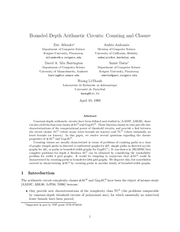10 Figure 1: G-graphs are important to the study of circuit complexity, since the reachability problem for width-k G-graphs is complete for depth-k AC0 [BLMS98]. Unfortunately, even for width-2 Ggraphs, counting the number of paths from s to t cannot be done in GapAC0. To see this, consider  2 1 . the small G-graph illustrated in Figure 1 which implements the reachability matrix A = 1 1 That is, there are two paths from vertex 1 (bottom row) in the first column to vertex 1 in the third column, and for all other (i, j) ∈ {1, 2}2 there is exactly one path from vertex i in the first column to vertex  column. Recall that all edges are directed from left to right. Note that  j in the third f2i+1 f2i i where fj denotes the j-th Fibonacci number. A = f2i f2i−1 Now consider the homomorphism h mapping σ ∈ {0, 1} to Aσ . Given a string x, the low-order bit of h(x)1,1 will be 0 if and only if the number of 1’s in x is equivalent to 1 (mod 3). Since the mod 3 function is not in AC0[2], it follows that counting the number of paths from s to t is not in GapAC0. A similar argument shows that this problem is complete for NC1 ACC0 reductions. Theorem 16 Counting the number of s-t paths in width-two G-graphs is complete for NC1 under ACC0 reductions. Proof: The group of two-by-two matrices with determinant 1 over the integers mod 5 is nonsolvable, and hence multiplication in it is hard for NC1 by [Ba89]. But given any multiplication in this group, we can construct path-counting problems in a G-graph whose answers modulo 5 are the entries of the product matrix. This is because any two-by-two matrix over N with determinant 1 can be represented as a product of those two matrices coded for by the columns of Figure 1. (For a proof of this fact, see, e.g., [Gu90, Theorem 3.1].) P Theorem 17 Define the σ-depth of a circuit to be the maximum number of gates on any path in the circuit. Arithmetic circuits of σ-depth k can be simulated by counting the number of s − t paths in a G-graph of width 2k + 2, where the subgraph between any pair of columns is drawn from the family illustrated in Figure 2. Conversely, given a G-graph G, the number of s − t paths in G can be computed by a uniform family of #AC0 circuits. 2 Proof: For the forward direction, we construct a function f which associates a graph f (C) with every gate C in a given #AC0 circuit, such that the number of s − t paths in f (C) is equal to the output of the gate. We assume, without loss of generality, that the circuit is leveled so that we can construct the function f by an induction on its depth. The construction uses the graphs Gk,j illustrated in Figure 2. C is the constant c: f (C) = Gk,c . C is the literal l: f (C) = Gk,l . 11 G 0,0 G G 0,1 G 0,2 k-1,i G k,i (0 ≤ i ≤ 2k) G k,,2k+1 Figure 2: The G-graphs Gi,j 12 G k,2k+2 Q C is a -gate at σ-depth d with inputs C1 , . . . , Cr : f (C) = f (C1 )Gk,2d+2f (C2 )Gk,2d+2 . . . Gk,2d+2f (Cr ) P C is a -gate at σ-depth d with inputs C1 , . . . , Cr : f (C) = Gk,2d+1 f (C1 )Gk,2d+1f (C2 ) . . . Gk,2d+1 f (Cr )Gk,2d+1 The G-graph for the formula (x1 x2 + x3 )(x2 + x1 x4 ) is illustrated in Figure 3. x1 x2 _ x2 _ x3 x1 x 4 Figure 3: G-graph for (x1 x2 + x3)(x2 + x1 x4) For a G-graph G of width 2k, let si (G), ti(G) (1 ≤ i ≤ 2k) denote the i-th vertex from the bottom on the left boundary and from the top on the right boundary, respectively. Thus with this convention, s = s1 (G) and t = t1 (G). We show that for a gate C at σ-depth d in the circuit, the number of sk−d (f (C)) − tk−d (f (C))-paths equals the value computed by C. The proof proceeds by induction on the height of the gate. Clearly G0,0 and G0,1 have respectively 0 and 1 s − t paths; and since Gk,i (for 0 ≤ i ≤ 2) is the same as G0,i when restricted to the two middle rows (and since there is no interference from any other row), the proposition holds true for literals and constants. Q If C is a -gate of σ-depth d, with input gates C1 , . . . , Cr , then each Ci has σ-depth d, hence by the inductive assumption, the value computed by Ci is the number of sk−d (f (Ci )) − tk−d (f (Ci )) paths. But for 1 ≤ i ≤ r − 1, tk−d (f (Ci )) and Qsk−d (f (Ci+1 )) are connected by an edge. Thus the number of sk−d (f (C))Q− tk−d (f (C)) paths is 1≤i≤r (number of sk −d (f (Ci )) − tk −d (f (Ci )) paths) which is the same P as 1≤i≤r (value computed by Ci ). If C is a -gate of σ-depth d, with input gates C1 , . . . , Cr , then each Ci has σ-depth d − 1, hence by the inductive assumption, the value computed by Ci is the number of sk−d+1 (f (Ci )) − tk−d+1 (f (Ci )) paths, which is same as the number of paths from sk−d to tk−d in the graph Gk,2d+1 f (Ci )Gk,2d+1 . Thus if we place the f (Ci )’s together with the Gk,2d+1’s between them, we get the sum of all such paths. Conversely, we have a width 2k graph g1′ . . . gn′ (where each gi′ is one of the Gk−1,j ’s illustrated in Figure 2) and we want to compute the number of s − t paths. First, we build the width 2k + 2 graph g0 . . . gn+1 , where g0 = Gk,2k+1 = gn+1 , and for 1 ≤ n, ′ if gi is Gk−1,j , then gi = Gk,j . This does not change the number of s − t paths, and makes the resulting algorithm easier to describe. Inductively, we define a number of functions σd [i, j] and πd [i, j], where 0 ≤ d ≤ k and 1 ≤ i < j ≤ n as follows 3 : 3  Pj−1  t=i+1 gt if gi , gj+1 ∈ {Gk,2 , Gk,3 } σ0 [i, j] = and gt ∈ {Gk,0, Gk,1} for i < t < j  1 otherwise Notice that we interpret the graphs Gk,0 and Gk,1 as the numerical constants 0 and 1. 13  Q ′ ′  i≤i′ <j ′ ≤j σ0[i , j ] if gi, gj+1 ∈ {Gk,3} π0 [i, j] = and gt ∈ {Gk,0 , Gk,1, Gk,2} for i < t < j  0 otherwise  P ′ ′  i≤i′ <j ′ ≤j πd−1 [i , j ] if gi, gj+1 ∈ {Gk,2d+2 , Gk,2d+3 } σd [i, j] = and gt ∈ {Gk,0 , . . . , Gk,2d+1} for i < t < j  1 otherwise  Q ′ ′  i≤i′ <j ′ ≤j σd [i , j ] if gi, gj+1 ∈ {Gk,2d+3 } πd [i, j] = and gt ∈ {Gk,0 , . . . , Gk,2d+2} for i < t < j  0 otherwise It is straightforward to show that πk [1, n] is the correct number of s − t paths. and that the functions defined above can indeed be computed by #AC0 circuits. Acknowledgment We thank Jin-Yi Cai for pointing us to [Gu90]. References [AAD97] M. Agrawal, E. Allender, S. Datta, On T C 0 , AC 0 and arithmetic circuits. In Proceedings of the 12th Annual IEEE Conference on Computational Complexity, pp:134–148, 1997. [ABFR91] J. Aspnes, R. Beigel, M. Furst, S. Rudich, The expressive power of voting polynomials. In Proceedings of the 23th ACM Symposium on Theory of Computing (STOC), pp:402–409, 1991. [ABL98] A. Ambainis, D. M. Barrington, H. LêThanh, On counting AC 0 circuits with negative constants. In Proceedings of the 23rd International Symposium on Mathematical Foundations of Computer Science (MFCS), 1998, pp:409–417. [ABO96] E. Allender, R. Beals, M. Ogihara, The complexity of matrix rank and feasible systems of linear equations. In Proceedings of the 28th ACM Symposium on Theory of Computing (STOC), pp. 161–167, 1996. [AJMV98] E. Allender, J. Jiao, M. Mahajan, and V. Vinay, Non-commutative arithmetic circuits: depth reduction and size lower bounds, Theoretical Computer Science, 209:47–86, 1998. [Al97] E. Allender, Making computation count: Arithmetic circuits in the nineties. In the Complexity Theory Column, edited by Lane Hemaspaandra, SIGACT NEWS 28, 4:2–15. [AJ93] C. Álvarez, B. Jenner, A very hard logspace counting class. Theoretical Computer Science, 107:3–30, 1993. 14 [AO96] E. Allender, M. Ogihara, Relationships among P L, #L and the determinant. In RAIROTheoretical Informatics and Applications Vol. 30, 1996, pp. 1–21. [Ba89] D. A. Barrington, Bounded-Width Polynomial-Size Branching Programs Recognize Exactly Those Languages in NC1. Journal of Computer and System Sciences 38(1):150–164, 1989. [BLMS98] D. M. Barrington, Ch-J Lu, P. B. Miltersen, S. Skyum, Searching constant width mazes captures the AC 0 Hierarchy. In Proceedings of the 15th Annual Symposium on Theoretical Aspects of Computer Science, 1998. [BRS91] R. Beigel, N. Reingold, D. Spielman, The perceptron strikes back. In Proceedings of the 6th Annual IEEE Structure in Complexity Theory Conference, 1991. [CMTV96] H. Caussinus, P. McKenzie, D. Thérien, H. Vollmer, Nondeterministic N C 1 Computation. In Proceedings of the 11th Annual IEEE Conference on Computational Complexity, pp:12–21, 1996. [DGS86] L. Denenberg, Y. Gurevich, and S. Shelah. Definability by constant-depth polynomial-size circuits. Information and Control, 70:216–240, 1986. [FFK94] S. A. Fenner, L. J. Fortnow, S. A. Kurtz, Gap-definable counting classes. Journal of Computer and System Science, 48(1):116–148, 1995. [Gu90] Y. Gurevich. Matrix decomposition Problem is complete for the average case. In Proceedings of the 31st Annual IEEE Symposium on Foundations of Computer Science (FOCS), pp:802–811, 1990. [Ha86] J. Hastad, Almost optimal lower bounds for small depth circuits. In Proceedings of the Eighteenth Annual ACM Symposium on Theory of Computing, pp:6–20, 1986. [FKPS85] R. Fagin, M. Klawe, N. Pippenger, and L. Stockmeyer. Bounded-depth, polynomial-size circuits for symmetric functions. Theoretical Computer Science, 36:239–250, 1985. [LêT98] H. LêThanh, Circuits Arithmétiques de Profondeur Constante, Thesis, Université Paris Sud, 1998. [Lu98] Ch. J. Lu, An exact characterization of symmetric functions in qAC 0 [2]. In Proceedings of the 4th Annual International Computing and Combinatorics Conference (COCOON), 1998. [MV97] M. Mahajan, V.Vinay, A combinatorial algorithm for the determinant. Proceedings of the Eighth Annual ACM-SIAM Symposium on Discrete Algorithms, pp:730–738, 1997. [NS98] F. Noilhan and M. Santha, Semantical Counting Circuits, submitted, 1998. [OH93] M. Ogiwara, L. Hemachandra, A complexity theory for feasible closure properties. Journal of Computer and System Sciences, 46(3):295–325, June 1993. [Ra87] A. A. Razborov, Lower bound on size of bounded depth networks over a complete basis with logical addition. Mathematicheskie Zametki, 41:598–607, 1987. English translation in Mathematical Notes of the Academy of Sciences of the USSR, 41:333–338, 1987. [Sm87] R. Smolensky, Algebraic methods in the theory of lower bounds for Boolean circuit complexity. In Proceedings of the 19th ACM Symposium on the Theory of Computing (STOC), pp:77–82, 1987. 15 [Tod92a] S. Toda, Counting problems computationally equivalent to the determinant. Manuscript. [Tod92b] S. Toda, Classes of arithmetic circuits capturing the complexity of computing the determinant. IEICE Transactions, Informations and Systems, E75-D:116–124, 1992. [Val79] L. Valiant, The complexity of computing the permanent. Theoretical Computer Science, 8:189–201, 1979. [Ven92] H. Venkateswaran, Circuit definitions of non-deterministic complexity classes. SIAM Journal on Computing, 21:655–670, 1992. [Vin91] V. Vinay, Counting auxiliary pushdown automata and semi-unbounded arithmetic circuits. In Proceedings of the 6th Annual IEEE Structure in Complexity Theory Conference, pp. 270– 284, 1991. 16