JUL 17, 2024
Tensor Parallelism in Three Levels of Difficulty


July 10, 2024
Whether it’s during training or at inference time, it’s often necessary to split models across multiple GPUs to get the most out of them. Tensor Parallelism is one such method for sharding models. Inspired by the excellent 5 Levels of Difficulty series, we explain Tensor Parallelism below in (just) three levels of difficulty: beginner, intermediate, and expert. By the time we get to the final stage, we will have built our own Tensor Parallelism implementation in PyTorch. Code accompanying this post can be found here.
Beginner
Neural networks operate on tensors, which are just large arrays of numbers. In the context of language models, an array is derived from sequences of words (such as sentences), where each word is represented by one or more slices of the array. This array is fed into a model that creates many similar arrays both internally and as its final output. If the model is a Large Language Model (LLM) and the input is a question, then the output array might contain an answer to that question (if it’s a good model).
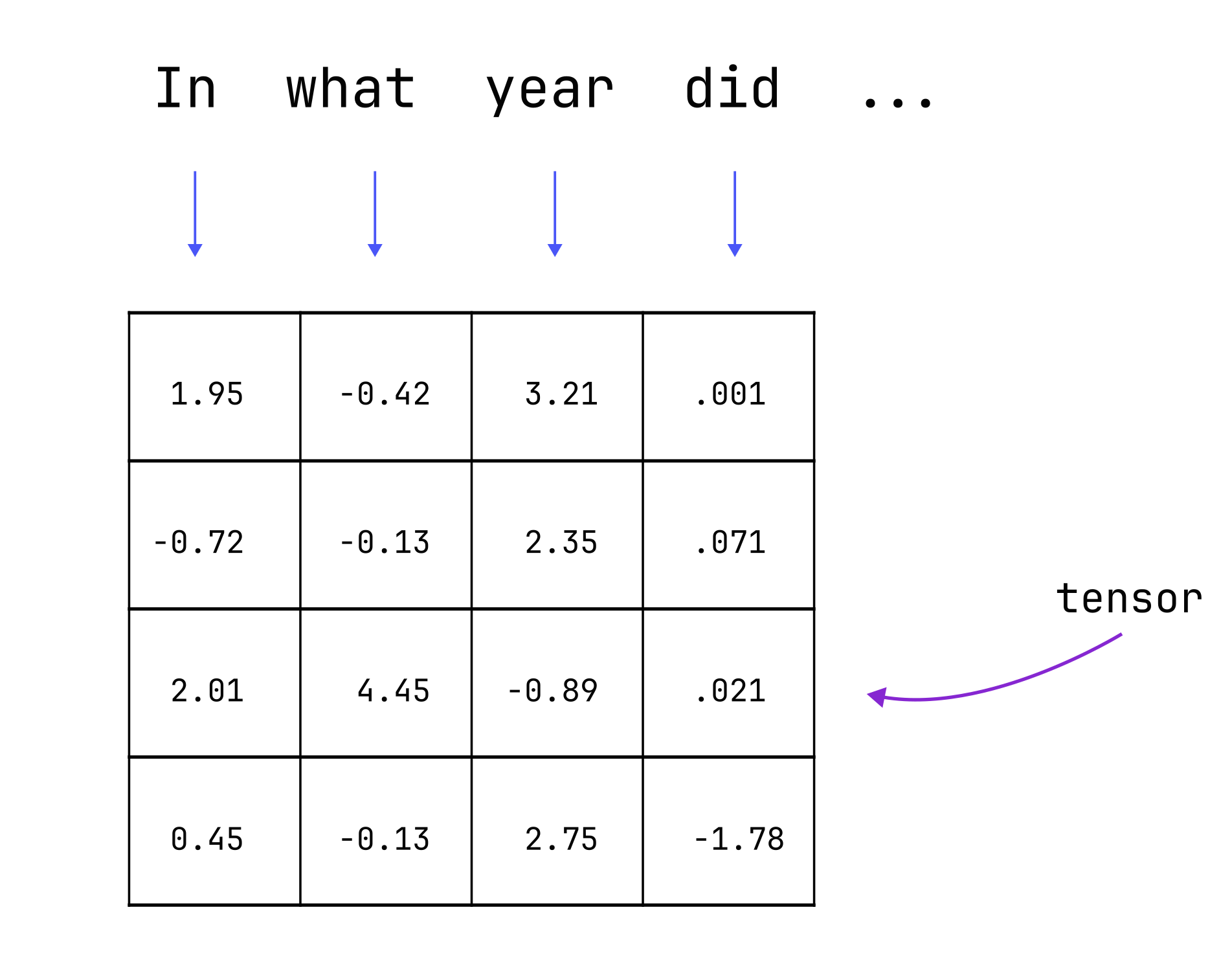
All of the numbers stored in these arrays take up memory on the Graphics Processing Unit (GPU), the hardware that neural networks run most efficiently on. The amount of memory required is determined by many factors including:
- The size of the input and output arrays.
- The number of inputs processed in parallel.
- The size of the model, which itself is built from arrays of numbers.
The larger any of these factors are, the higher the GPU memory requirement. Exactly how much memory is needed depends on whether the model is being trained, or just used (commonly called “inference”), but in both cases, it is easy to run out of GPU memory.
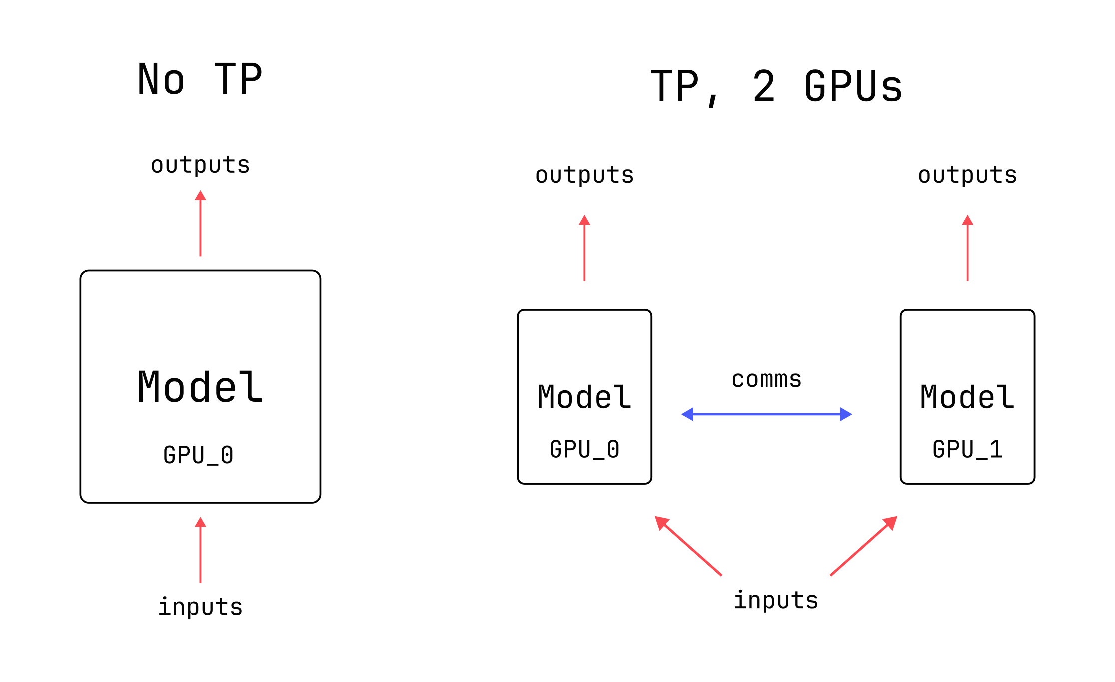
In order to avoid running out of memory, we can use multiple GPUs at once and make use of their combined memory. This requires splitting the various arrays across machines and getting the GPUs to cooperate with each other. There are many ways to do this splitting, also known as “sharding”. Some methods break apart the input arrays, while others break apart the arrays that the model itself is built from (also known as “weights”). Tensor Parallelism is a splitting strategy which breaks apart the model weights, as well as the intermediate arrays that the model generates.
There is no free lunch, though: Tensor Parallelism can be complicated to implement and it generally results in each GPU being used less efficiently. Primary reasons for this include the coordination between machines and the fact that GPUs generally work better when operating on larger sets of numbers. Nevertheless, it is one of the best options for splitting up a model that won’t fit into GPU memory, particularly at inference time.
Intermediate
Tensor Parallelism (TP) splits tensors along the model’s hidden dimension in order to reduce per-GPU memory costs. Using multiple GPUs with TP enables larger per-GPU batch sizes and is commonly used during inference for this reason.
The splitting is typically implemented via pairs of Linear layers, where the first instance
performs the sharding and the second one unshards the result. We will use the Transformer MLP layer
as a case study. You, having intermediate-level experience with LLMs, might already be familiar with
this layer, but we will give a refresher, just in case.
The MLP inputs are (batch_size, seq_len, d_model)-shaped, where d_model is the size of the
model’s hidden dimension. Three operations are performed:
- The inputs are expanded via a matrix-multiply to shape
(batch_size, seq_len, 4 * d_model) - The expanded tensor is passed through a non-linear function, say
nn.GELU. - The tensor is shrunk back down to shape
(batch_size, seq_len, d_model)via a matrix-multiply.
A minimal PyTorch implementation is below.
class MLP(nn.Module):
    """
    Basic MLP (multi-layer perceptron) layer. Dropout is neglected.
    """

    def __init__(
        self,
        d_model: int,
        device: Optional[Union[str, torch.device]] = None,
        dtype: Optional[torch.dtype] = None,
    ) -> None:
        super().__init__()

        self.lin_0 = nn.Linear(
            d_model,
            4 * d_model,
            device=device,
            dtype=dtype,
        )
        self.act_fn = nn.GELU()
        self.lin_1 = nn.Linear(
            4 * d_model,
            d_model,
            device=device,
            dtype=dtype,
        )

    def forward(self, inputs: torch.Tensor) -> torch.Tensor:
        x = self.lin_0(inputs)
        x = self.act_fn(x)
        x = self.lin_1(x)
        return x
A Tensor Parallel version of the MLP layer splits up the two matrix-multiplies above across multiple
GPUs. This results in smaller matrices in the two nn.Linear layers,
as well as smaller intermediate tensors consumed and produced in step 2 above.
For example, let’s say our batch_size, seq_len, and d_model are 16, 2048, and 4096 respectively. Then, without Tensor Parallelism, the various tensor and layer shapes are:
- Input:
(16, 2048, 4096). - 1st
Linear:(16384, 4096). - Output of the 1st
Linear:(16, 2048, 16384). - 2nd
Linear:(4096, 16384). - Output of the 2nd
Linear:(16, 2048, 4096).
With Tensor Parallelism on 2 GPUs, the shapes on each GPU are:
- Input:
(16, 2048, 4096). - 1st
Linear:(8192, 4096). - Output of the 1st
Linear:(16, 2048, 8192). - 2nd
Linear:(4096, 8192). - Output of the 2nd
Linear:(16, 2048, 4096).
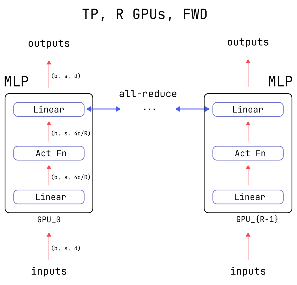
Notice that in the Tensor Parallel version, the inputs to the MLP layer and the final outputs are not reduced in size: at the end of the computation, every GPU is left with tensors of the same size as the non-Tensor-Parallel version. However, populating each GPU’s tensors with the correct values requires communication, because each GPU only has access to a part of the computation.
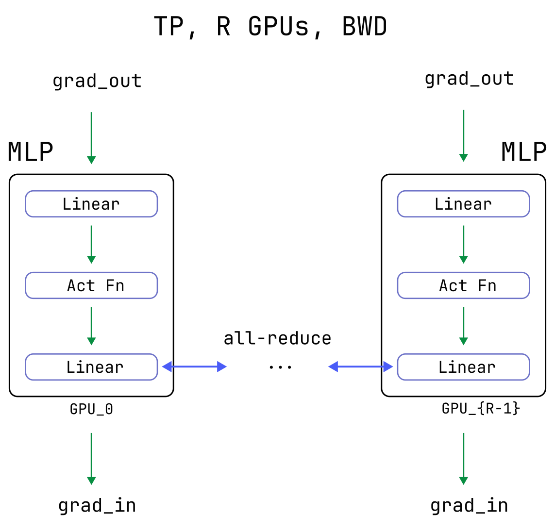
Specifically, at the end of the computation each GPU needs to add the partial results from all other GPUs to their own partial result. During training, additional communication is needed during the backward pass in order to compute gradients correctly. More details can be found in the Megatron-LM paper. Below is a diagram of the Tensor Parallelism forward pass with two GPUs.

The main advantage of Tensor Parallelism is that it reduces the memory cost of the large weights in
the Linear layers by the number of GPUs which are used, as well as the large “activation” tensors
which are created in the middle of the MLP layer and are saved during training (see this
post for a deep dive on the costs of activation memory).
Tensor Parallelism also reduces the overall time of the computation.
The disadvantage of Tensor Parallelism is that it generally reduces GPU efficiency, for two primary reasons:
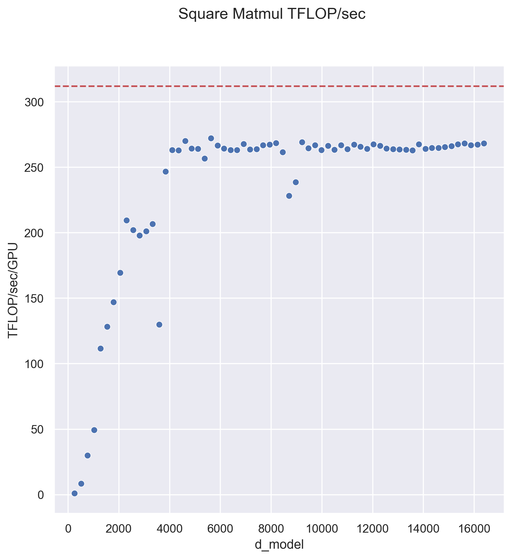
- The communications between GPUs need to be completed before the model can move forward, which can seriously hamper efficiency. Nobody likes waiting around.
- Modern GPUs often achieve higher throughput when performing larger matrix-multiplies (see the plot below), but Tensor Parallelism unfortunately reduces the size of the matrix-multiplies.
Tensor Parallelism is just one strategy among many for distributed computation, and keeping the dizzying array of options straight can be difficult. To help with this, the following table indicates which quantities are sharded for some common strategies:
| batch dim | sequence dim | hidden dim | weights | optimizer | |
| Data Parallel | ✔ | ||||
| Tensor Parallel | ✔ | ✔ (intra-layer) | ✔ | ||
| Sequence Parallel + TP | ✔ | ✔ | ✔ (intra-layer) | ✔ | |
| RingAttention | ✔ | ||||
| Pipeline Parallel | ✔ (inter-layer) | ✔ | |||
| ZeRO-1 & 2 | ✔ | ✔ | |||
| FSDP/ZeRO-3 | ✔ | ✔ (intra-layer) | ✔ |
Above, intra-layer means that individual weights in a layer are sharded across GPUs, while inter-layer means that each layer is kept intact, but different layers are placed on different GPUs. The first three columns indicate the dimensions along which the activations are sharded, if any.
Expert
Tensor Parallelism can be used to shard all of the large weight matrices in a model, which also has the consequence of sharding some of the intermediate activations. Critical-path collective communications between GPUs are needed to correctly perform this sharding, and so Tensor Parallelism is typically restricted to high-bandwidth, single node domains, with other parallelization strategies reserved for cross-node sharding.
Tensor Parallelism plays different roles in inference and training.
- TP is extremely common for inference because its memory reductions allow for larger KV-cache sizes, which can greatly improve efficiency. Tensor parallelism is particularly well-suited to inference architecturally, because only the activations are communicated around (unlike FSDP/ZeRO3, which would communicate weights for every newly-generated token) and every rank is involved in every step of the computation (unlike Pipeline parallelism, in which GPUs would necessarily idle).
- During training, TP reduces memory costs from gradients, optimizer state, and activations, in addition to its parameter memory savings. However, TP is rarely used by itself for model training, due to the relatively high costs of its blocking collectives. Pipeline parallelism, the ZeRO strategies, and FSDP are typically better choices, with Tensor Parallelism layered on top when memory constraints require it.
In the following sections, we prove the correctness of Tensor Parallelism for the Transformer MLP
layer, build out a minimal torch implementation, and perform some profiling.
Math and Correctness
Tensor Parallelism relies on the basic fact that sums can be performed in any order. We first show how this fact is leveraged for the forward pass, and then discuss the implications for the backward pass.
NOTE
The forward-pass section is heavily mathy, but in the end it’s all about rearranging sums. Keep the dot-product in mind as a simpler example. Let’s say we have two
(16, )-shaped tensors,xandy. Their dot-product can be computed asdot = x @ y = (x * y).sum(). If we rearranged the tensors to have shapes(2, 8)as inx_reshape = x.reshape(2, 8)and similar fory_reshape, we could also compute this asdot = (x_reshape * y_reshape).sum(); the rearrangement doesn’t matter, we just have to sum over everything. We then Tensor-Parallelize the computation by dividing the sums across machines. Using two GPUs, we could place the(8, )-shaped shardx_shard = x_reshape[0]on one GPU,x_shard = x_reshape[1]on the other, do similarly fory_shard, and run the following on each GPU:# Compute locally available sums first dot = (x_shard * y_shard).sum() # Or x_shard @ y_shard # Complete remaining sums via communication torch.distributed.all_reduce(dot)The final value of
dotin all cases is the same. The math below is just a more general version of the above concept.
Forward Pass
Start by succinctly writing out the entire MLP computation in Einstein notation, whose details we expand upon below.
\[\begin{align} z _{ bsd } &= W ^{ 1 }_{ d e } \,\phi \left ( W ^{ 0 } _{ e d' } x _{ bsd' } + B ^{0} _{e}\right ) + B ^{ 1 } _{ d } \end{align}\]With these conventions, repeated indices are implicitly summed over, which greatly declutters
expressions. See e.g. torch.einsum
or the einops package for code implementations.
Above, \(x _{ bsd }\) is the MLP input where \(b\), \(s\), and \(d\) index the batch, sequence position, and hidden dimension, respectively. The output \(z _{ bsd }\) has the same shape as the input, and \(\phi\) is a generic, element-wise non-linearity. The learnable weight and bias parameters are capitalized and have shapes
\[W ^{ 0 } _{ ed' } \in \mathbb{R} ^{ 4 \texttt{d_model}\times \texttt{d_model} } \ , \quad B ^{0}_{ e} \in \mathbb{R} ^{ 4 \texttt{d_model}}\\ W ^{ 1 } _{de} \in \mathbb{R} ^{ \texttt{d_model}\times 4\texttt{d_model} } \ , \quad B ^{1}_{ d} \in \mathbb{R} ^{ \texttt{d_model}} \ .\]Any sum above (i.e. any repeated index) can be computed in any order. Equivalently, any summed-over index can be arbitrarily reshaped. For the MLP TP computation, it is most advantageous to reshape the length \(4 \texttt{d_model}\) \(e\)-index into a pair of indices \(r, f\), of respective sizes \(R\) (which will be the number of ranks the layer is sharded over) and \(4 \texttt{d_model}/R\), and write the computation in the equivalent form
\[\begin{align} z _{ bsd } &= W ^{ 1 }_{ d e } \,\phi \left ( W ^{ 0 } _{ e d' } x _{ bsd' } + B ^{0} _{e}\right ) + B ^{ 1 } _{ d }\\ &= W ^{ 1 }_{ d rf} \,\phi \left ( W ^{ 0 } _{ rf d' } x _{ bsd' } + B ^{0} _{rf}\right ) + B ^{ 1 } _{ d } \end{align}\]Tensor Parallelism performs the MLP computation in the second form above, placing tensors with different \(r\)-indices on different GPUs. There are two stages:
- Each GPU computes the sum over the \(f\)-dimension using its locally available \(r\)-shards. For
example, when using four GPUs, the
rank = 3GPU would perform its forward pass with the \(r=3\) slice of the large weight \(W ^{ 0 } _{ rf d' }\), a shard of shape(4 d_model // R, d_model), withR = 4here. - The sum over the \(r\)-index is performed by an all-reduce, completing the calculation and populating the final output on all machines.
The above, two-line correctness proof for the TP MLP forward pass only relies on the fact that sums
can also be reshaped in the presence of an intervening element-wise operation, \(\phi\). torch
tests of these manipulations in the simpler case of a dot-product can be found
here
(local tests) and
here
(distributed tests).
The takeaway is that Tensor Parallelization is fairly simple, conceptually: just reshape a summed-over index and perform the sharded computation across multiple machines using collective communications to complete the sums. Split your sums and invent your own parallelization strategy today!
Backward Pass
There is only one subtlety for achieving backward-pass correctness: an additional all-reduce is needed. This is true for any operation which uses unsharded inputs to produce a sharded-output.
The all-reduce is needed in the general case where a neural network is used to compute a scalar loss \(L\) and there exists some intermediate operation which takes an unsharded tensor \(x\) (indices omitted) and creates a sharded tensor \(y _{ r }\), with \(r\) indexing the GPU on which \(y _{ r }\) resides. That is, \(y _{ r } = F \left ( x, \ldots \right)\) where the operation \(F\) may also depend on arbitrarily many other tensors, sharded or not.
The backward pass requires computing the partial derivative \(\frac{ \partial L }{\partial x }\). By the chain rule, this is given by
\[\frac{ \partial L }{ \partial x }=\sum_{r} \frac{ \partial L }{ \partial y_r } \frac{ \partial y_r }{ \partial x }\]where we have made the sum over ranks explicit. Due to the sharding, each rank only has access to the data necessary to compute a single term in the sum, \(\frac{ \partial L }{ \partial y_r } \frac{ \partial y_r}{ \partial x }\) for their value of \(r\), and so the sum needs to be completed via an all-reduce.
In the context of the MLP layer, this applies to the output from the first sharded matrix-multiply above:
\[y _{ srf } \equiv W ^{ 0 } _{ rf d } x _{ sd } + B ^{0} _{rf}\]After computing the local gradients with respect to the inputs \(x\), an all-reduce across ranks populates their true, global value.
NOTE
No additional collectives or other considerations are needed to pass backwards through the all-reduce which was done in the forward pass. This is because an all-reduce is a simple sum of the form \(z = \sum_{r} y_{r}\), and so the corresponding chain-rule factor is just the identity for each rank: \(\frac{ \partial z }{ \partial y_r }=1\).
Implementation
Implementing TP in torch requires writing custom autograd.Fuction classes in order to correctly
backpropagate through the collectives described above. We need the following two functions,
which are used in the forward- and backward-pass collectives described above, respectively:
class AllReduceFwdIdentityBwd(torch.autograd.Function):
    @staticmethod
    def forward(
        ctx: Any, inputs: torch.Tensor, group: dist.ProcessGroup
    ) -> torch.Tensor:
        inputs = inputs.clone()
        dist.all_reduce(inputs, group=group)
        return inputs

    @staticmethod
    def backward(ctx: Any, grad_outputs: torch.Tensor) -> tuple[torch.Tensor, None]:
        return grad_outputs, None


class IdentityFwdAllReduceBwd(torch.autograd.Function):
    @staticmethod
    def forward(
        ctx: Any, inputs: torch.Tensor, group: dist.ProcessGroup
    ) -> torch.Tensor:
        ctx.group = group
        return inputs

    @staticmethod
    def backward(ctx: Any, grad_outputs: torch.Tensor) -> tuple[torch.Tensor, None]:
        grad_outputs = grad_outputs.clone()
        dist.all_reduce(grad_outputs, group=ctx.group)
        return grad_outputs, None
Even though AllReduceFwdIdentityBwd has essentially the same behavior as its underlying
all_reduce collective, the autograd.Function wrapper is still advisable: omitting the wrapper
raises a backward-pass UserWarning due to c10d::allreduce_ not having a registered autograd
kernel and will raise an error in future torch versions.
NOTE
Similar
autograd.Functioncollectives do exist in the PyTorch repo undertorch.distributed.nn.functional, but, for some reason, they do not appear in the official documentation and largely haven’t been touched in years.
Using the above functions, we now build two Linear subclasses: one which produces sharded outputs
and one which consumes sharded inputs. These will replace the first and second Linear layers in
the non-TP MLP class, respectively.
class LinearShardedOutputs(nn.Linear):
    """
    Generates sharded outputs from unsharded inputs.

    Input shape:
        (batch_size, seq_len, in_features)
    Output shape:
        (batch_size, seq_len, out_features // group.size())
    """

    def __init__(
        self,
        in_features: int,
        out_features: int,
        group: dist.ProcessGroup,
        device: Optional[Union[str, torch.device]] = None,
        dtype: Optional[torch.dtype] = None,
    ) -> None:
        sharded_out_features, remainder = divmod(out_features, group.size())
        assert not remainder, "out_features must be divisible by the ProcessGroup size"
        super().__init__(
            in_features=in_features,
            out_features=sharded_out_features,
            device=device,
            dtype=dtype,
        )

        self.group = group

    def forward(self, inputs: torch.Tensor) -> torch.Tensor:
        # Wrap the unsharded inputs for backwards-pass correctness.
        x = IdentityFwdAllReduceBwd.apply(inputs, self.group)
        x = super().forward(x)
        return x


class LinearShardedInputs(nn.Linear):
    """
    Generates unsharded outputs from sharded inputs.

    Input shape:
        (batch_size, seq_len, in_features // group.size())
    Output shape:
        (batch_size, seq_len, out_features)
    """

    def __init__(
        self,
        in_features: int,
        out_features: int,
        group: dist.ProcessGroup,
        device: Optional[Union[str, torch.device]] = None,
        dtype: Optional[torch.dtype] = None,
    ) -> None:
        sharded_in_features, remainder = divmod(in_features, group.size())
        assert not remainder, "in_features must be divisible by the ProcessGroup size"
        super().__init__(
            in_features=sharded_in_features,
            out_features=out_features,
            device=device,
            dtype=dtype,
        )
        self.group = group

    def forward(self, inputs: torch.Tensor) -> torch.Tensor:
        x = inputs @ self.weight.T
        # All-reduce the matmul output for forwards-pass correctness.
        x = AllReduceFwdIdentityBwd.apply(x, self.group)
        # Crucial: add the bias _after_ the all-reduce.
        x = x + self.bias
        return x
These correspond to simplified versions of the ColumnParallelLinear and RowParallelLinear
layers
of Megatron-LM, respectively.
The Tensor Parallel MLP layer can then be written as a subclass of the non-TP layer by simply
swapping out the Linear instances. No need to change the forward method:
class MLPTP(MLP):
    """
    Basic Tensor Parallel MLP (multi-layer perceptron) layer. Dropout is neglected.

    Input and output shapes:
        (batch_size, seq_len, d_model)
    Intermediate activation shapes:
        (batch_size, seq_len, 4 * d_model // group.size())
    """

    def __init__(
        self,
        d_model: int,
        group: Optional[dist.ProcessGroup] = None,
        device: Optional[Union[str, torch.device]] = None,
        dtype: Optional[torch.dtype] = None,
    ) -> None:
        nn.Module.__init__(self)
        # Fallback to the WORLD process group, if None provided
        group = group or dist.group.WORLD

        self.lin_0 = LinearShardedOutputs(
            d_model,
            4 * d_model,
            group=group,
            device=device,
            dtype=dtype,
        )
        self.act_fn = nn.GELU()
        self.lin_1 = LinearShardedInputs(
            4 * d_model,
            d_model,
            group=group,
            device=device,
            dtype=dtype,
        )
All of the layer implementation code can be found here, along with correctness tests.
Some final implementation notes:
- Tensor Parallel self-attention layers are built in nearly identical ways: the
Linearlayer which generates the queries, keys, and values is replaced by aLinearShardedOutputsinstance, and the finalLinearprojection layer is replaced by aLinearShardedInputs. The number of attention heads processed per rank is reduced by the Tensor Parallelism degree. - If it bothers you that the intermediate activations are sharded, but the MLP inputs and outputs are not, take a look at Sequence Parallelism.
- An exciting new PyTorch
DTensorAPI is under development which aims to provide convenient abstractions for distributing computations with less work.
Performance and Profiling
Last, let us discuss performance characteristics and profile the throughput for the forward pass of
a long-ish sequence in, say, bfloat16, as occurs during training or the pre-fill stage at inference
time. There are a few fundamental quantities at play:
- The total floating point operations (FLOPs) needed per TP group, approximately: \(16\times\texttt{batch_size}\times \texttt{seq_len}\times \texttt{d_model} ^{ 2}\)
- The bytes communicated in the all-reduce: \(4\times\texttt{batch_size}\times \texttt{seq_len}\times \texttt{d_model} \times (R-1) / R\)
- The achievable FLOPs/sec/GPU: \(\lambda_{\rm GPU}\)
- The achievable communication bandwidth: \(\lambda_{\rm comms}\) in Bytes/s.
The last two factors implicitly depend on \(\texttt{batch_size}\), \(\texttt{seq_len}\), and \(\texttt{d_model}\), but in practice once the tensor sizes get large (think ~ O(100MiB)) both factors approach approximately constant values.
Tensor Parallelism is efficient if the communication time is decently smaller than the computation time:
\[t_{\rm comms} = \frac{4\times\texttt{batch_size}\times \texttt{seq_len}\times \texttt{d_model} \times (R-1)}{R\times\lambda_{\rm comms}}\\ t_{\rm GPU} = \frac{16\times\texttt{batch_size}\times \texttt{seq_len}\times \texttt{d_model} ^{ 2}}{R \times \lambda_{\rm GPU}}\]yielding a ratio (which we want to minimize) of
\[\frac{ t_{\rm comms}}{t_{\rm GPU} }= \frac{ R-1 }{ \texttt{d_model} } \times \frac{ \lambda_{\rm GPU}}{ 4 \,\lambda _{ \rm comms }} \ .\]The analysis above is only approximate, but the general lessons are correct: Tensor Parallelism typically becomes more costly as the number of TP ranks \(R\) increases, but gets cheaper as the hidden dimension grows. These trends can be seen in the plot below, which was measured on a single 8xA100 node using the code presented in this post:

In practice, the costs of TP can be less severe than what is demonstrated here where all
measurements have batch_size = 1, as the TP memory savings will typically be leveraged to process
larger batch sizes which generally run more efficiently.
Conclusion
Tensor Parallelism is an indispensable tool for running large models, both during inference and training. Whether you just need to know the basics or require the nitty gritty details, we hope this introduction to Tensor Parallelism was informative. Many implementations of Tensor Parallelism exist in the PyTorch ecosystem, and all of them can be easily run using Determined AI, a general-purpose platform for distributed deep learning. Join our Slack channel or email us to discuss how to run your advanced distributed workload on Determined today!
Recent Posts
JUL 02, 2024