In the ever-evolving world of data analysis, mastering the top Excel formulas and functions is essential for maximizing productivity and efficiency. As we move into 2024, Excel remains a cornerstone tool for professionals across industries, from finance to marketing so for a better output you have to learn using Excel formulas. Whether you’re a seasoned analyst or a beginner, exploring the excel formula list below will significantly boost your data handling capabilities.

From the indispensable VLOOKUP and INDEX MATCH to the versatile XLOOKUP and FILTER, these formulas are designed to streamline your workflow and enhance data accuracy. Imagine effortlessly summarizing data with SUMIFS, managing conditional logic with IF and IFS, or performing complex calculations with ARRAYFORMULA. These essential Excel formulas are not just tools but gateways to smarter, faster, and more reliable data management.
Before going through into the excel formulas list, it’s crucial to distinguish between formulas and top excel functions as there is always queries related to excel formulas vs functions. Formulas, initiated with the equal sign (=), are the foundation for performing intricate calculations, while functions are predefined operations with names indicating their specific utility. This exploration of Excel’s formula landscape promises to enhance the proficiency of both beginners and seasoned users, unlocking the full potential of this versatile spreadsheet software.
You can use Excel formulas to find patterns in the values in your spreadsheet’s cells, conduct calculations on those values, and then return the results to the cell of your choice. Some basic Excel formulas include those for sum, subtraction, percentage, division, average, even dates and times, and a lot more.
For example: =A1+A2+A3+A4+A5, which finds the sum of the range of values from cell A1 to cell A5.
What is an Excel Function
Where a formula in Excel is a mathematical expression that computes the value of a cell, functions in Excel are already existing preset formulas in Excel. Based on the values supplied as arguments or parameters, functions perform certain calculations in a specific order. Every time using Excel formulas there are many questions such as what does this formula mean in excel, what does excel formula mean all will be resolved.
For example: =SUM (A1:A10). This function adds up all the values in cells A1 through A10.H
How to Use Functions in Excel
In the most recent versions of Excel, you may discover and enter Excel formulas into particular cells of your spreadsheet by navigating to the top menu bar and clicking on Formulas and selecting the type of formula.
Quick Tip to Become a Pro in Excel: The more you use Excel formulas, the easier it will be to remember and perform them manually. Excel has over 400 functions, and the number is increasing from version to version. The formulas can be inserted into Excel using the following method:
Step 1: Open your Excel Sheet and Choose a cell.
Step 2: Type “=”, then press Enter.
Step 4: Enter an operator.
Step 6: Press Enter.

Insert Function
The simplest way to insert fundamental Excel formulas is by typing a formula into a cell or the formula bar. Typically, the process begins with typing an equal sign (=) followed by the name of an Excel function, by doing this Excel will start showing you suggestions in the drop down menu to select and enter the formula.
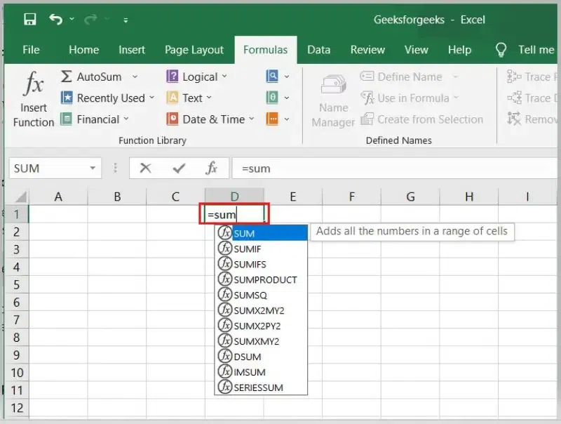
Simple Insertion by Typing the Formula in Excel
If you want complete control over your function insertion, use the Excel Insert Function dialogue box. To do so, go to the Formulas tab and select the first menu, Insert Function. All the functions will be available in the dialogue box.
.webp)
Using the Insert Function option from Formulas Tab in Excel
This option is for those who want to quickly dive into their favorite functions. Navigate to the Formulas tab and select your preferred group to access this menu. Click to reveal a sub-menu containing a list of functions. You can then choose your preference. If your preferred group isn’t on the tab, click the More Functions option — it’s most likely hidden there.
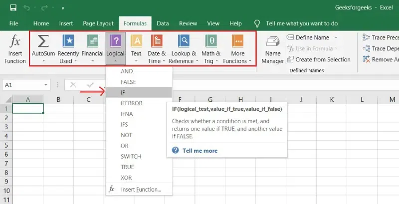
Selecting the Formula from Formula Tab in Excel
4. Using Quick Insert to use Recently Used Tabs in Excel
If retyping your most recent formula becomes tedious, use the Recently Used menu. It’s on the Formulas tab, the third menu option after AutoSum.
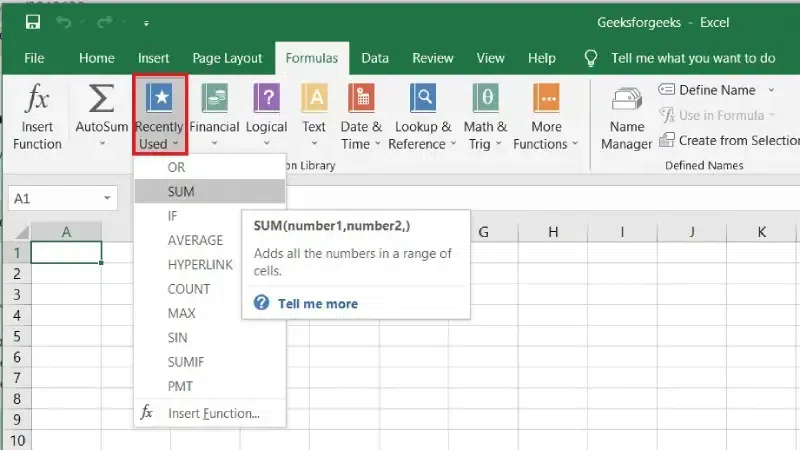
Recently Used Tabs
|
Term
|
Description
|
Example
|
|
Formula
|
A specific expression that calculates a value based on input values. Formulas can be simple (e.g., =A1 + B1) or complex (e.g., =VLOOKUP(A1, A2:B10, 2, FALSE))
|
=A1 + B1
|
|
Function
|
A pre-built formula that performs a specific task. Examples of functions include SUM, AVERAGE, COUNT, etc. Functions can take multiple arguments (inputs) and return a single output value.
|
=SUM(A1:A10)
|
The SUM formula in Excel is one of the most fundamental formulas you can use in a spreadsheet, allowing you to calculate the sum (or total) of two or more values. To use the SUM formula, enter the values you want to add together in the following format: =SUM(value 1, value 2,…..).
Example: In the below example to calculate the sum of price of all the fruits, in B9 cell type =SUM(B3:B8). This will calculate the sum of B3, B4, B5, B6, B7, B8 Press “Enter,” and the cell will produce the sum: 430.
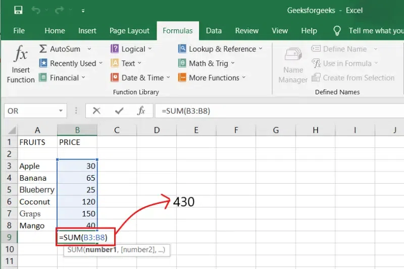
Excel SUM Formula
To use the subtraction formula in Excel, enter the cells you want to subtract in the format =SUM (A1, -B1). This will subtract a cell from the SUM formula by appending a negative sign before the cell is subtracted.
Example: If A3 was 300 and B3 was 225, =SUM(A1, -B1) would perform 300 + -225, returning a value of 75 in D3 cell.
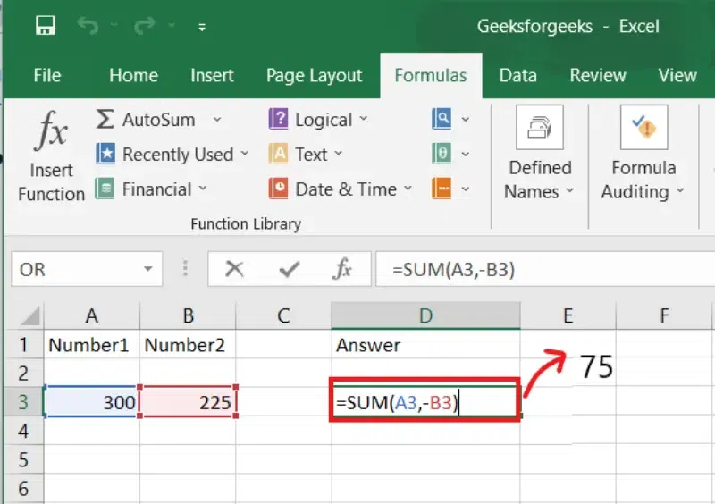
Excel SUBTRACTION Formula
In Excel, enter the cells to be multiplied in the format =A3*B3 to perform the multiplication formula. An asterisk is used in this formula to multiply cell A3 by cell B3.
Example: If A3 was 300 and B3 was 225, =A1*B1 would return a value of 67500.
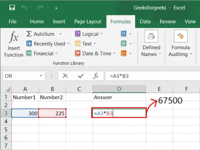
Excel MULTIPLICATION Formula
Highlight an empty cell in an Excel spreadsheet to multiply two or more values. Then, in the format =A1*B1…, enter the values or cells you want to multiply together. The asterisk effectively multiplies each value in the formula.
To return your desired product, press Enter. Take a look at the screenshot above to see how this looks.
4. Excel DIVISION Function
Division in Excel is one of the most basic functions available. To do so, highlight an empty cell, enter an equals sign, “=,” and then the two (or more) values you want to divide, separated by a forward slash, “/.” The output should look like this: =A3/B3, as shown in the screenshot above. To use the division formula in Excel, enter the dividing cells in the format =A3/B3. This formula divides cell A3 by cell B3 with a forward slash, “/.”
Example: If A3 was 300 and B3 was 225, =A3/B3 would return a decimal value of 1.333333333.
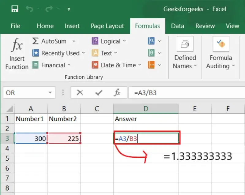
Excel DIVISION Function
5. Excel AVERAGE Function
The AVERAGE function finds an average or arithmetic mean of numbers. To find the average of the numbers, type = AVERAGE(A3, B3, C3….) and press ‘Enter’ it will produce the average of the numbers in the cell.
Example: If A3 was 300, B3 was 225, C3 was 180, D3 was 350, E3 is 400 then =AVERAGE(A3,B3,C3,D3,E3) will produce 291.
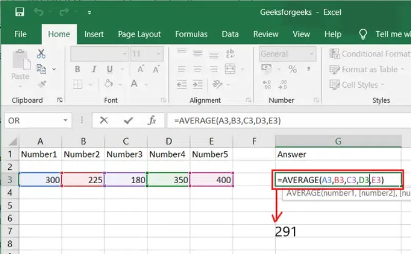
Excel AVERAGE Function
6. Excel IF () Function
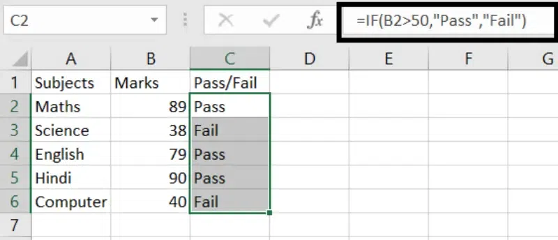
In Excel, the IF formula is denoted as =IF(logical test, value if true, value if false). This lets you enter a text value into a cell “if” something else in your spreadsheet is true or false.
Example: You may need to know which values in column A are greater than three. Using the =IF formula, you can quickly have Excel auto-populate a “yes” for each cell with a value greater than 3 and a “no” for each cell with a value less than 3.
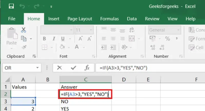
Excel IF () Function
To use the percentage formula in Excel, enter the cells you want to calculate the percentage for in the format =A1/B1. To convert the decimal value to a percentage, select the cell, click the Home tab, and then select “Percentage” from the numbers dropdown.
Excel doesn’t have a set “formula” for percentages, but it makes it simple to transform any cell’s value into a %, saving you the time and effort of having to compute and reenter the data.
On Excel’s Home tab, you can find the default setting for converting a cell’s value to a percentage. Select this tab, highlight the cell(s) you want to convert to a percentage, and then select Conditional Formatting from the dropdown menu (this menu button might say “General” at first). Then, from the list of options that appears, choose “Percentage.” This will convert the value of each highlighted cell into a percentage. You can find this functionality lower down.
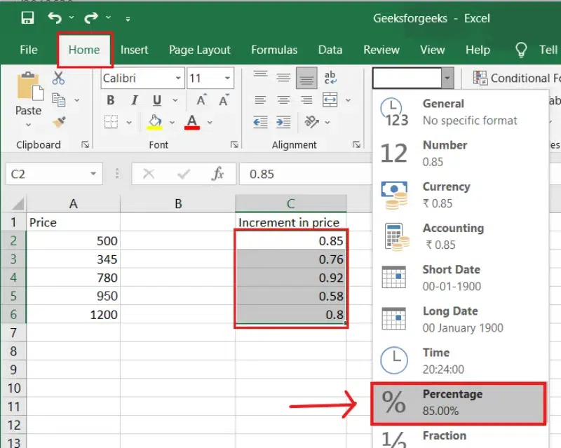
Excel PERCENTAGE Formula
8. Excel MODULUS Function
The MOD() function aims to return the remaining after dividing a given number by a divisor. For a better understanding, let’s look at the examples below.
Example: We have divided 20 by 3. The remainder is calculated using the function “=MOD(A2,3)”. The outcome is kept in B2. Alternatively, we can just type “=MOD(20,3)” and get the same result.
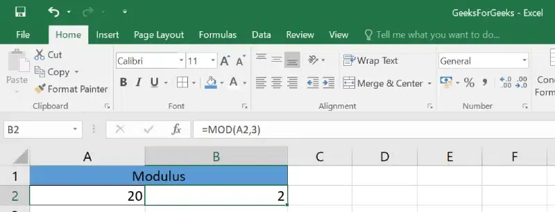
Excel MODULUS Function
CONCATENATE is a useful formula that combines values from multiple cells into the same cell.
Example: =CONCATENATE(A3,B3) will combine Red and Apple to produce RedApple.
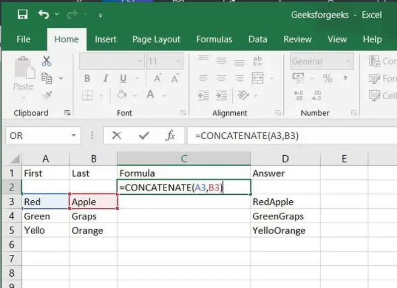
Excel CONCATENATE Formula
DATE is the Excel DATE formula =DATE(year, month, day). The values entered in the parenthesis, including values from other cells, will be converted to a date using this formula.
Example: If A2 was 2019, B2 was 8, and C1 was 15, =DATE(A1,B1,C1) would return 15-08-2019.
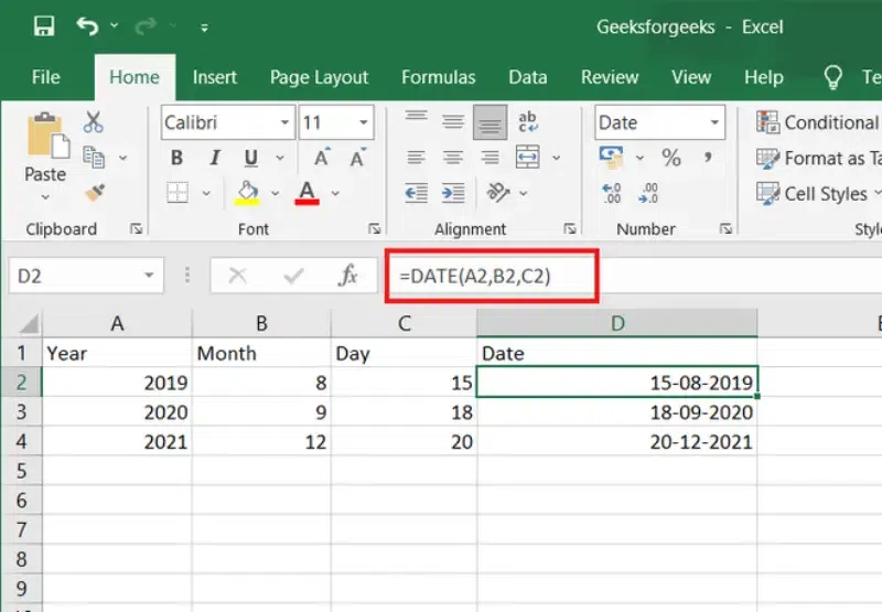
Excel DATE Formula
The TRIM formula in Excel is denoted =TRIM(text). Any spaces placed before or after the text in the cell will be eliminated by this formula.
Example: If A2 includes the name “Virat Kohli” with unwanted spaces before the first name, =TRIM(A2) would return “Virat Kohli” with no spaces in a new cell.
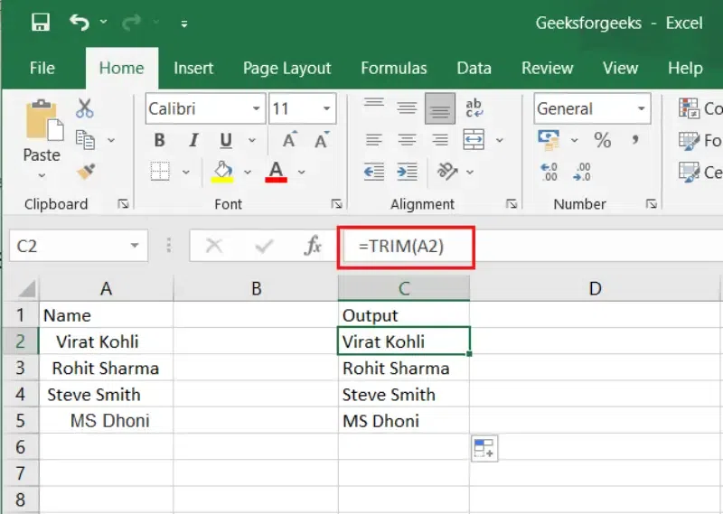
Excel TRIM Formula
12. Excel LEN Function
LEN is the function to count the number of characters in a specific cell when you want to know the number of characters in that cell. =LEN(text) is the formula for this. Please note that Excel’s LEN function counts every character, including spaces.
Example: =LEN(A2), returns the total length of the character in cell A2, including spaces.
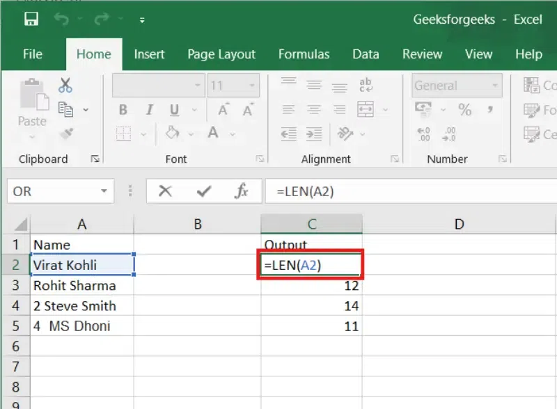
Excel LEN Function
13. Excel CEILING Function
In ceiling a number is rounded up to the nearest multiple of importance using the CEILING() function.
Example: The nearest highest multiple of 1 for 2.5 is 3.
Note: The #VALUE! error value is returned by CEILING if either input is not a number.
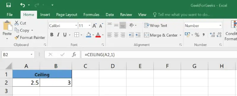
Excel CEILING Function
14. Excel FLOOR Function
The floor function reduces a number to the nearest multiple of importance, in contrast to the ceiling function.
Example: The nearest lowest multiple of 1 for 2.5 is 2.
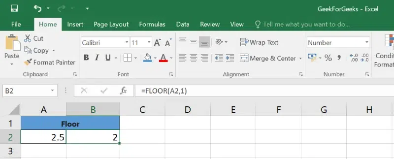
Excel FLOOR Function
15. Excel REPLACE Function
The REPLACE() function does exactly what its name implies, it replaces a portion of a text string with another text string.
The syntax is =REPLACE(old_text, start_num, num_chars, new_text).
- Old_text: Text in which you want to replace some characters.
- Start_num in this case refers to the index position from which you wish to begin replacing the characters. The amount of characters you want to replace is then indicated by num_chars.
- New_text: The text that will replace characters in old_text.
Example: =REPLACE(A3,3,2,”23″) Replaces the last two digits (22) of 2022 with 23 making it 2023.
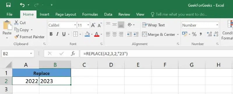
Excel REPLACE Function
Example: =REPLACE(A2,1,5,”@”) Replaces five characters in GeeksForGeeks with a single @ character, starting with the first character (G).
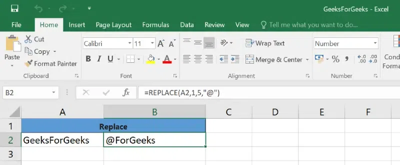
Excel REPLACE Function
16. Excel SUBSTITUTE Function
In a text string, the SUBSTITUTE() function substitutes new text for old text.
Syntax: SUBSTITUTE(text, old_text, new_text, [instance_num])
Text: The text or the reference to a cell containing text for which you want to substitute characters.
Old_text: The text you want to replace.
New_text: The text you want to replace old_text with.
[instance_num] refers to the index position of the present texts more than once.
Example: =SUBSTITUTE(A2, “Student”, “Employee”) Substitutes Employee for Student (Employee Details) making it Employee Details.
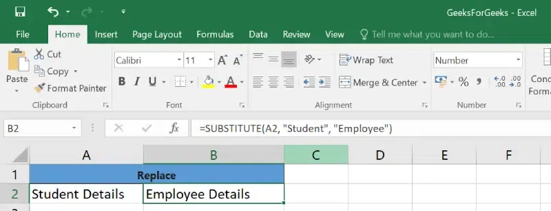
Excel SUBSTITUTE Function
17. Excel NOW() Function
The NOW() function in Excel give the present date (today’s date), It retrieves the current system clock time.
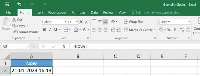
Excel NOW() Function
18. Excel TODAY() Function
The TODAY() function in Excel provides the current system date.
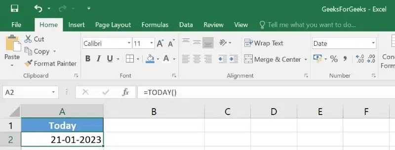
Excel TODAY() Function
19. Excel DAY() Function
The function DAY() is used to return the day of the month. The value will fall between 1 and 31. The first day of the month is 1 and the last day is 31.
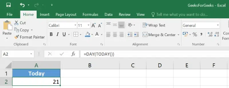
. Excel DAY() Function
20. Excel MONTH() Function
The month is returned by the MONTH() function as a number between 1 and 12, with 1 denoting January and 12 denoting December.
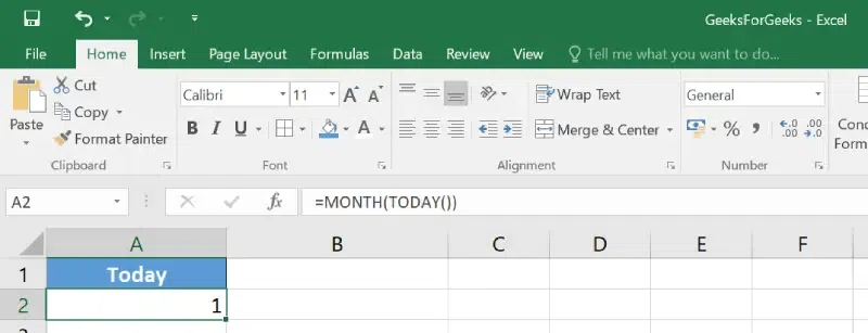
Excel MONTH() Function
21. Excel YEAR() Function
The YEAR() function, as the name suggests, returns the year from a date value.
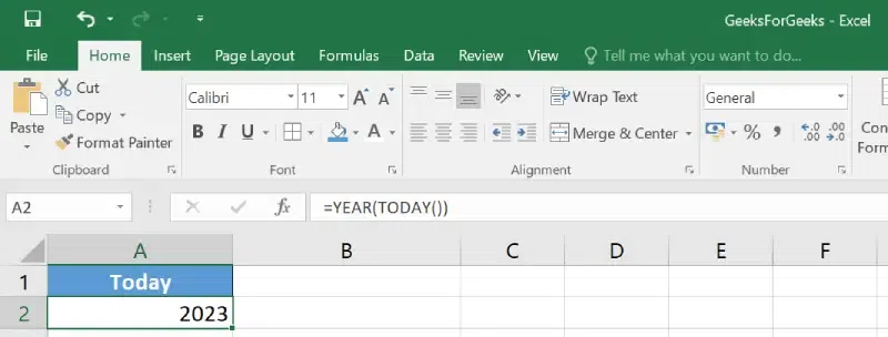
Excel YEAR() Function
22. Excel TIME() Function
The Excel serial number with a time format is created by the TIME() function using the hours, minutes, and seconds provided as numbers.
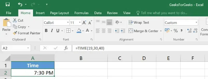
Excel TIME() Function
23. Excel DATEDIF Function
The DATEDIF() function provides the difference between two dates in terms of years, months, or days.
Example: Using DATEDIF function to calculate the current age of a person based on two given dates, the date of birth and today’s date.
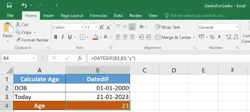
Excel DATEDIF Function
The VLOOKUP formula searches for the value in the leftmost column of the table array and returns the value from the same row from the specified columns.
Formula: =VLOOKUP(lookup_value, table_array,col_index, range_lookup)
Lookup_value: The value for which you are looking.
Table_array: the range of the table, worksheet, or selected cell with multiple columns.
col_index: The position of the column to extract the value.
range_lookup: “TRUE” indicates the approximate match(default), and “FALSE” indicates the exact match.
Example: =VLOOKUP(A10,A1:C7,2,FALSE)
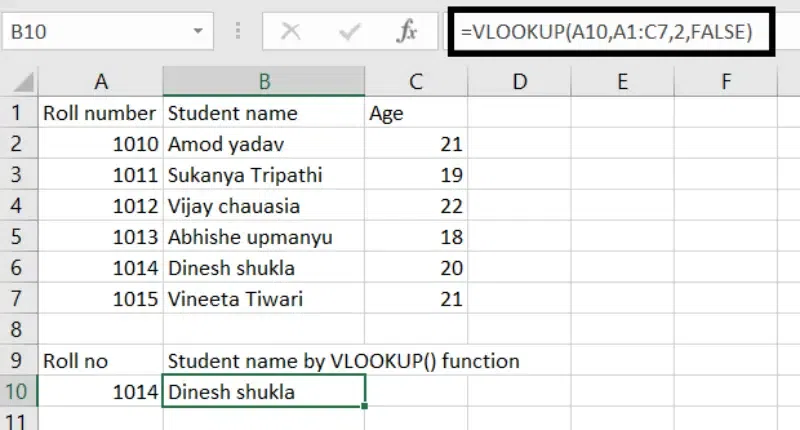
Excel VLOOKUP Formula
HLOOKUP(Horizontal lookup) is similar to the VLOOKUP formula. This function looks for a value in the top row of a table or array of benefits. It gives the value in the same column from a row you specify.
Formula: =HLOOKUP(lookup_value, table, row_index, range_lookup)
Lookup_value: This indicated the value for lookup.
Table_array: the range of the table, worksheet, or selected cell with multiple columns.
row_index: The position of the row to extract the value.
range_lookup: “TRUE” indicates the approximate match(default), and “FALSE” indicates the exact match.
Example: HLOOKUP(B5,A1:D3,3,0)
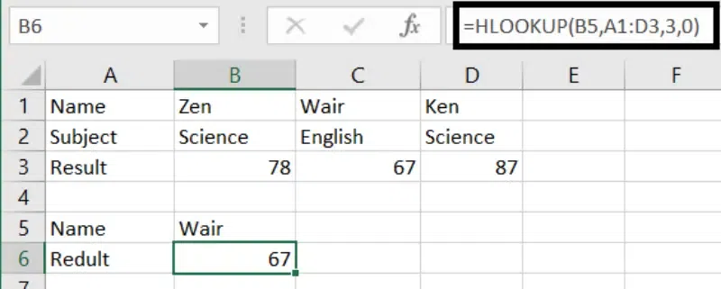
Excel HLOOKUP Formula
26. Excel POWER Function
The POWER() function returns the result of a number raised to a certain power.
Formula: POWER(number, power)
Example: POWER(A2,3)
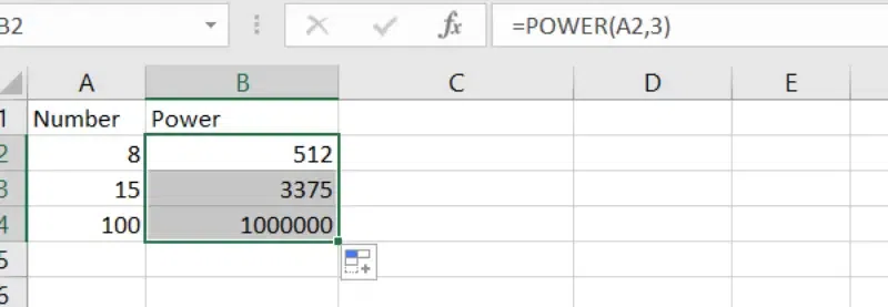
Excel POWER Function
27. Excel INDEX-MATCH Function
The INDEX-MATCH function can be used to return a value in a column to the left. This is the most popular function in Excel for performing more advanced lookups. INDEX-MATCH in Excel has several advantages over the VLOOKUP Function. The main advantage of using INDEX-MATCH is it only has to consider the lookup column and the return column.
Formula: INDEX(reference, [row], [column])
Example: =INDEX(B2:B6,MATCH(D2,A2:A6,0))
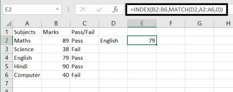
Excel INDEX-MATCH Function
28. Excel Data Analysis Function
What-If Analysis involves altering values to test various scenarios within Advanced Excel.
Multiple sets of values can be applied to one or more formulas in Advanced Excel to explore diverse outcomes.
Solver is a valuable tool for What-If Analysis, functioning as an add-in program in Microsoft Excel. It helps identify optimal values for a formula within a designated cell, known as the objective cell. However, constraints or limits may apply to other formula cell values on a worksheet.
Solver operates with decision variables, which are cell groups used in calculating formulas within objective and constraint cells. It adjusts the values of decision variable cells to adhere to constraints on constraint cells, assisting in determining the desired outcome for the objective cell.
Excel Data Analysis Function
29. Excel SUMIF() Function
SUMIF Function adds all the values in a range of cells that meet a specified condition.
Formula: = SUMIF(range,criteria,[sum_range]).
Example: = SUMIF(C6:C11,”>=20″)
30. Excel AVERAGEIF() Function
It Calculates the average value in a range of cells that meet the specified criteria. Formula: =AVERAGEIF(range,criteria,[average_range]).
Example: =AVERAGEIF(C6:C11,”>=20″)
31. Excel COUTNIF() Function
The COUNTIF Function is used to count the total number of cells in the given range that satisfy the condition.
Formula: COUNTIF(range, criteria)
Example: =COUNTIF(C2:C6,”PASS”)
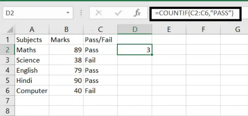
Excel COUTNIF() Function
32. Offset Function in Excel
The OFFSET function retrieves a reference to a cell range located a defined number of rows and columns away from a given cell or range of cells.
Offset Function =OFFSET(reference, rows, cols, [height], [width])
Conclusion
In conclusion, mastering the top Excel formulas and functions in 2024 is crucial for anyone looking to enhance their data analysis skills and boost productivity. Whether it’s the powerful XLOOKUP, the versatile INDEX MATCH, or the efficient SUMIFS, these tools provide unmatched flexibility and precision in managing data. By incorporating these essential Excel functions into your workflow, you’ll be well-equipped to handle complex data tasks with ease and accuracy.
How to use the COUNTIF function in excel?
Follow the steps given below to use COUNIF Function in Excel:
- Select the Cell
- Enter the Formula
- Press Enter
Here are the 7 functions of Excel formulas:
- Mathematical Functions
- Statistical Functions
- Text Functions
- Date and Time Functions
- Lookup and Reference Functions
- Logical Functions
- Financial Functions
How to Use LOOKUP Function in Excel?
To use the LOOKUP Function in Excel follow the steps given below:
- Select the Cell
- Enter the LOOKUP Formula
- Press Enter
- Calculation Performed
Follow the below steps to insert formulas in Excel:
- Step 1: Select the cell where you want the output
- Step 2: Type (=) sign followed by Formula.
For example: To sum two values put “=A1+A2”.
Yes, We can use multiple formulas by nesting. Nesting is using one formula and inside another. Nesting allows us to perform complex problems.
For example, if you want to multiply two vlaues you can use Multiply function on the basis of a given condition using the IF function.