0% found this document useful (0 votes)
42 viewsLecture10 Regression2 TS PDF
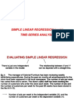
(1) The manager of Colonial Furniture analyzed weekly advertising expenditures and store sales over 26 weeks. The number of newspaper ads placed (independent variable X) ranged from 1 to 7, while the number of customers (dependent variable Y) varied from week to week. (2) A scatter plot of X and Y showed a weak positive linear relationship. The regression line estimated that for each additional ad, sales would increase by 21 customers. (3) However, ads explained only 8.5% of variation in customers. Most variation remained unexplained.
Uploaded by
snoozermanCopyright
© © All Rights Reserved
Available Formats
Download as PDF, TXT or read online on Scribd
0% found this document useful (0 votes)
42 viewsLecture10 Regression2 TS PDF
(1) The manager of Colonial Furniture analyzed weekly advertising expenditures and store sales over 26 weeks. The number of newspaper ads placed (independent variable X) ranged from 1 to 7, while the number of customers (dependent variable Y) varied from week to week. (2) A scatter plot of X and Y showed a weak positive linear relationship. The regression line estimated that for each additional ad, sales would increase by 21 customers. (3) However, ads explained only 8.5% of variation in customers. Most variation remained unexplained.
Uploaded by
snoozermanCopyright
© © All Rights Reserved
Available Formats
Download as PDF, TXT or read online on Scribd
/ 22