2. ph250b.14 measures of association 1

Measures of association learning objectives
1. Define and understand the difference between the concepts of “effects” and
“associations”
2. Use a contingency (2x2) table to organize information on disease occurrence
in time
3. Understand the differences between the additive and multiplicative scales
a. Identify the scale of each measure of association
4. Know how to calculate and interpret measures of association listed below
(this includes knowing the formulas)
a. Relative measures
i. Cumulative incidence ratio
ii. Incidence density ratio
iii. Prevalence ratio
iv. Odds ratio
b. Absolute measures
i. Attributable risk (aka risk difference)
ii. Attributable risk percent
iii. Population attributable risk
iv. Population attributable risk percent
c. Number needed to treat
5. Understand what the strength of an association captures
6. Understand what relative and absolute measures capture
7. Understand what attributable percentage measures capture

Measures of association outline
– Big picture
– Scales of measures
– The 2x2 table
– Measures of association
• Relative measures
• Absolute measures
• Other measures
– Summary

Big picture
• In epidemiology, we often compare measures of
disease frequency between different groups
– Building on measures of disease module
• Typically comparing disease frequency between
groups with different exposures
• The goal is to ascertain associations between
exposures and outcomes and, ultimately, effects
of exposures on outcomes

Big picture
• Reminder on the distinction between
associations and effects
• An association tells us about probabilities of past
events
– Carrying matches is associated with lung cancer

Big picture
• An effect is causal and it tells us how
probabilities change if conditions change
– If you remove matches from pockets in the
population, does the rate of lung cancer decrease?
?

Big picture
• Measures of association quantify the strength
and direction of associations between exposures
and outcomes
• Strength of association:
– Is exposure weakly related to outcome? Strongly?

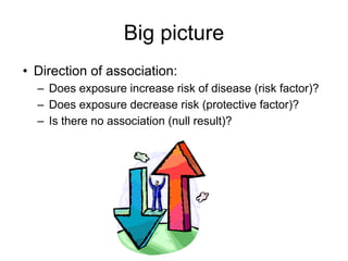
Big picture
• Direction of association:
– Does exposure increase risk of disease (risk factor)?
– Does exposure decrease risk (protective factor)?
– Is there no association (null result)?

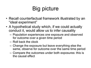
Big picture
• Recall counterfactual framework illustrated by an
“ideal experiment”
• A hypothetical study which, if we could actually
conduct it, would allow us to infer causality
– Population experiences one exposure and observed
for outcome over a given time period
– Roll back the clock
– Change the exposure but leave everything else the
same, observe for outcome over the same time period
– Compare the outcomes under both exposures: this is
the causal effect

Big picture
• In reality, the “ideal experiment” cannot be conducted
• We evaluate the associations between exposures and
outcomes by comparing outcomes between groups that
experienced different exposures

Big picture
• Measure of association does not necessarily (or
even typically) quantify a causal effect
• Associations may be explained by various
sources:
– Causal relation
– Chance (random error)
– Bias (systematic error)

Big picture
• Throughout course will enumerate the methods
for:
– Designing studies to minimize error (systematic and
random)
– Assessing the roles of systematic and random error
once a study is conducted (qualitatively and
quantitatively)
– Incorporating knowledge or assumptions about the
causal process
– Analytically removing or adjusting for error to the
extent possible

Big picture
• These are key steps to moving towards inferring
causality from associations

Measures of association outline
– Big picture
– Scales of measures
– The 2x2 table
– Measures of association
• Relative measures
• Absolute measures
• Other measures
– Causal perspective on scales and measures
– Summary

Scales of measures
• There are different scales for measuring
associations between variables
• Analogy: if you wanted to measure weight
changes you might measure:
– Weight loss/gain in lbs
– Weight loss/gain as a percentage of starting weight
– Change in BMI percentile
• Comparison of gain/loss between people would
depend on measure used

Scales of measures
• Similarly, there are different scales for
quantifying the size or strength of association
between an exposure and an outcome

Scales of measures
• Measures of association can be calculated on
two different scales:
– Relative scale (ratios)
– Absolute scale (differences)
• Each scale has several defining characteristics:
– Range of values that the measure of association can
take
– Null value: value at which there is no association
(value consistent with the null hypothesis of no
association)

Scales of measures
• The scale of a measure of association is critical
because measures on different scales capture
different things
• First focus on learning how the scales are
different
• We will discuss motivations for choosing relative
versus absolute measures towards the end of
this module

Scales of measures
Relative scale – ratio measures of association
• The ratio of two measures of diseases is on the
relative scale:
– Example: (rate among the exposed)/(rate among the
unexposed)
– IDexposed
/ IDunexposed
• Examples of relative measures include:
Cumulative incidence ratio (CIR), incidence
density ratio (IDR)
• The CIR and IDR are often referred to as risk
ratio or rate ratio respectively, and are
abbreviated RR

Scales of measures
Relative scale – ratio measures of association
• Range: zero to positive infinity
• Null value: 1
• CIR = 1 or IDR = 1 means the exposure is not
associated with the outcome

Scales of measures
Absolute scale – difference measures of
association
• The difference between two measures of
disease is on the absolute scale:
– Example: rate among the exposed – rate among the
unexposed
– IDexposed
– IDunexposed
• Examples of absolute measures include:
attributable risk/rate (AR), population attributable
risk/rate (PAR)
• Note that “attributable risk” often used
generically to include risks and rates

Scales of measures
Absolute scale – difference measures of
association
• Range: negative infinity to positive infinity
• Null value: 0
• AR = 0 means the exposure is not associated
with the outcome

2x2 table
• Count data is typically organized with a 2x2 or contingency table
• Example: with incidence data a/(a+b) = CIe
• What is CI in the total population?

2x2 table
• Incidence density data is also organized with a 2x2 or contingency
table
• Example: a/PTe
= IDe

2x2 table
• Note that Stata and the Kleinbaum text book present the
table “backwards” with exposure on top and disease on
the left
• Pay attention to the orientation of the table before
making calculations

2x2 table
Note on notation
– PTexposed
= PTe
– PTunexposed
= PTu
– PTtotal
= PTt
– Will also see applied to measures of disease including
CI, ID

Relative measures
• Measures to be discussed
– Risk/rate ratio
– Prevalence ratio
– Odds ratio

Relative measures
• Risk/rate ratio (RR) – aka relative risk
– “Risk” in relative risk used generically to include risk or rate
• Provides information about relative association between
an exposure and a disease
• The risk/rate of disease in the exposed is compared to
the same measure among the unexposed as a ratio
• RR = Rexposed
/ Runexposed
= Re
/ Ru
• Where R indicates either risk or rate – (i.e., CI
(cumulative incidence) or ID (incidence density))

Relative measures
• RR can be used to refer generically to these relative
measures
• CIR is the specific term when cumulative incidence is
used
• IDR is the specific term when incidence density is used
• Used to see term RR used generically for any relative
measure (including OR, PR) but current trend is toward
specific terms

Relative measures
• Interpretations of RR:
• Relative difference in the risk/rate of disease between
the exposed and unexposed
• Interpretation of RR=5: Risk/rate of disease in the
exposed is 5 times the risk/rate in the unexposed
• Interpretation of RR=0.5: Risk/rate of disease in the
exposed is 0.5 times the risk/rate in the unexposed

Relative measures
• Example: study of oral contraceptive (OC) use and
bacteriuria among women 16-49 yrs
over 1 year
• RR = ?
• What measures of disease incidence can we estimate
from this data?
• How do we compare them to estimate RR?

Relative measures
• Can estimate CIs
• Take ratio to estimate RR
• RR = CIR = CIe
/CIu
=
• RR = (27/482)/(77/1908) = 1.39
• Women who use OCs have 1.39 times the risk of
bacteriuria (over 1 year) compared with women who do
not use OCs
• Note that as with CI, CIR is only interpretable with
information on the time period over which it was
calculated

Relative measures
• Prevalence ratio (PR)
an exposure and a disease, using prevalence as the
measure of disease
– Analogous to RR
• PR = Prevexposed
/ Prevunexposed
= Preve
/ Prevu

Relative measures
• Interpretations of PR:
• Relative difference in the prevalence of disease
between the exposed and unexposed
• Interpretation of PR=5: Prevalence of disease among
the exposed is 5 times the prevalence in the unexposed
• Interpretation of PR=0.5: Prevalence of disease in the
exposed is 0.5 times the prevalence of disease in the
unexposed

Relative measures
• A brief aside on odds
• Odds – two equivalent definitions
– Odds = number of people with event / number of people without
an event
– Odds = probability of event occurring / probability of event not
occurring = P / (1-P)
• Example:
– 10 people in a classroom of 50 have a cold
– Probability of having a cold = 10/50 = 0.2
– Probability of not having a cold = 40/50 = 0.8
– Odds of having a cold = 10/40 = 0.2/0.8 = 0.25
• Odds range from 0 to positive infinity

Relative measures
• Utility of odds will become apparent when we discuss
study design and analysis of epidemiologic data
– When a disease is rare, odds can be modeled in place of risks
with similar results
– In some study designs (case-control varieties) odds estimate
pseudo-risks/rates (more in study design)

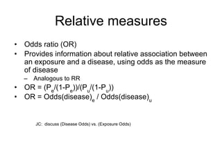
2. ph250b.14 measures of association 1

Relative measures
• Odds ratio (OR)
an exposure and a disease, using odds as the measure
of disease
– Analogous to RR
• OR = (Pe
/(1-Pe
))/(Pu
/(1-Pu
))
• OR = Odds(disease)e
/ Odds(disease)u
JC: discuss (Disease Odds) vs. (Exposure Odds)

Relative measures
• Interpretations of OR:
• Relative difference in the odds of disease between the
exposed and unexposed
• Interpretation of OR=5: Odds of disease is in the
exposed is 5 times the odds in the unexposed
• Interpretation of OR=0.5: The odds of disease in the
exposed is 0.5 times the odds of disease in the
unexposed
• Note: it is incorrect to interpret the odds ratio as the
risk/rate ratio
– Exception for particular case-control study designs (more in
study design module)

Relative measures
• OR always more extreme than RR (further from null)
– When the disease is rare the values will be close
– Note that this is not relevant for designs in which OR captures a
risk/rate ratio directly (more in study design)

Relative measures
• OR versus RR
• Example:
– Recall the example of students having a cold
• P=0.2
• Odds=0.25
– Say we wanted to compare this classroom to an office
– In the office, 10 out of 100 people have a cold.
• P = 10/100 = 0.1
• Odds = 10/90 = 0.111
– Exposed are students, unexposed are office workers, outcome
is cold
– RR comparing students to workers: RR = 0.2 / 0.1 = 2
– OR comparing students to workers: OR = 0.25 / 0.111 = 2.25

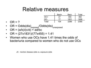
Relative measures
• OR = ?
• OR = Odds(dis)exposed
/Odds(dis)unexposed
• OR = (a/b)/(c/d) = ad/bc
• OR = (27x1831)/(77x455) = 1.41
• Women who use OCs have 1.41 times the odds of
bacteriuria compared to women who do not use OCs
JC: mention disease odds vs. exposure odds

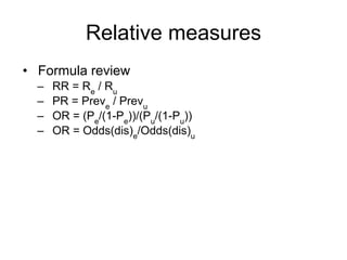
Relative measures
• Formula review
– RR = Re
/ Ru
– PR = Preve
/ Prevu
– OR = (Pe
/(1-Pe
))/(Pu
/(1-Pu
))
– OR = Odds(dis)e
/Odds(dis)u

Relative measures
• Exercise for home (discuss in lab)
• Hypothetical RCT for injection drug users
– Primary outcomes are cessation of drug use
– HIV as a secondary outcome of interest

Relative measures
• Exercise at home / in lab
• 60 people randomized to a 12-month residential
detoxification program
– 49 tested HIV negative at the start of the trial
– At the end of the trial, 5 participants tested positive
for HIV who had been negative at the start of the trial
• 60 people randomized to 12-months of
outpatient treatment

Relative measures
• Exercise at home / in lab
• Calculate and interpret relative measures of
association of potential interest from these trial
results

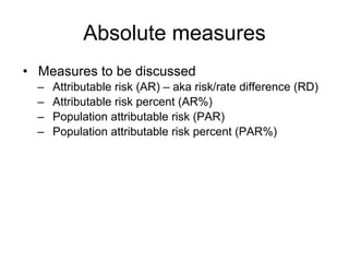
Absolute measures
• Measures to be discussed
– Attributable risk (AR) – aka risk/rate difference (RD)
– Attributable risk percent (AR%)
– Population attributable risk (PAR)
– Population attributable risk percent (PAR%)

Absolute measures
• Attributable risk (AR) – aka risk/rate difference (RD)
• “Risk” in attributable risk used generically to include risk
or rate
• Provides information about absolute association
between an exposure and a disease, or the excess risk
or rate of disease in the exposed
• AR = Rexposed
– Runexposed
• Where R indicates either risk or rate – (i.e., CI
(cumulative incidence) or ID (incidence density))

Absolute measures
• Interpretations of AR:
• Difference in risk/rate of disease between the exposed
and unexposed
• Excess risk/rate of disease in the exposed compared
with the unexposed
• AR has same units as the incidence measure used (risk
(dimensionless) if CI; rate (1/time) if ID)

Absolute measures
Szklo Figure 3-1

Absolute measures
• Example: study of oral contraceptive (OC) use and
bacteriuria among women 16-49 yrs
over 1 year
• AR = ?
• How do we compare cumulative incidence to estimate
AR?

Absolute measures
• Take difference to estimate AR
• AR = CIe
– CIu
=
• AR = (27/482)–(77/1908) = 0.01566
• Women who use OCs have 0.01566 higher risk of
bacteriuria compared with women who do not use OCs
over 1 year
• Can multiply by a population size to facilitate
interpretation: 0.01566x100,000 = 1566/100,000
• Among every 100,000 women who use OCs there are
1566 excess cases of bacteriuria compared with women
who do not use OCs over 1 year

Absolute measures
• Attributable risk percent (AR%)
• Provides information about the excess incidence in the
exposed (AR) as a percentage of incidence in the
exposed population
• AR% = (Rexposed
– Runexposed
) / Rexposed
x 100
• AR% = AR/ Rexposed
x 100

Absolute measures
• Interpretations of AR%:
• Percentage of all disease incidence among the exposed
that is associated with the exposure
• Percentage of disease incidence in the exposed that is
in excess of the incidence in the unexposed

Absolute measures
Szklo Figure 3-1
100% of incidence
in the exposed
population AR% - percentage of
disease incidence in
the exposed that is in
excess of the
incidence in the
unexposed

Absolute measures
• AR% = ?
• AR% = (CIe
– CIu
)/CIe
x 100
• AR% = (27/482)–(77/1908)/(27/482) x 100 = 28%
• Of the bacteriuria incidence among women who use
OCs, 28% is in excess of the incidence in women who
do not use OCs

Absolute measures
• Attributable risk percent (AR%) is analogous to efficacy
for an intervention (e.g., vaccine, other treatment)
• The control group is considered “exposed”
• The treatment group is considered “unexposed”
• AR% = (Rexposed
– Runexposed
) / Rexposed
x 100
• Efficacy% = (Rcontrol
– Rtreatment
) / Rcontrol
x 100
• Percentage of disease incidence in the control group
that is in excess of the incidence in the treatment group

Absolute measures
• Population attributable risk (PAR)
• Provides information about the excess risk or rate of
disease in the entire population (not just among the
exposed as with AR)
– Sometimes the AR is called the “attributable risk among the
exposed” to make this distinction clear
• PAR = Rtotal
– Runexposed
• Alternative formulation:
• PAR = (AR)(Pe
)
– Pe
= prevalence of the exposure in the total population
– See extra slides for derivation
• Alternative formulation useful if estimating PAR for a
total population other than your study population for
which you have an estimate of Pe

Absolute measures
• Interpretations of PAR:
• Excess risk/rate of disease in the total population
compared with the unexposed
• If association is believed to be causal, PAR can be used
to estimate the impact of an exposure on the health of a
population of interest
• PAR will never be larger than AR in a given population
• PAR has same units as the incidence measure used
(risk (dimensionless) if CI; rate (1/time) if ID)

Absolute measures
• PAR = ?
• PAR = CIt
– CIu
=
• PAR = (104/2390)–(77/1908) = 0.00316
• In the total population of women there is 0.00316 higher
risk of bacteriuria compared with women who do not
use OCs
• Can multiply by a population size to facilitate
interpretation: 0.00316x100,000 = 316/100,000
• There are 316 excess cases of bacteriuria for every
100,000 women in the total population compared with
women who do not use OCs
JC: review NNT

Absolute measures
• Comparison of AR and PAR
• AR = 1566/100,000
• PAR = 316/100,000
• PAR < AR
• Why is this the case?

Absolute measures
• Population attributable risk percent (PAR%)
• Provides information about the excess incidence in the
total population (PAR) as a percentage of incidence in
the total population
• PAR% = (Rtotal
– Runexposed
) / Rtotal
x 100
• PAR% = (PAR / Rtotal
) x 100

Absolute measures
• PAR% = ?
• PAR% = (CIt
– CIu
)/CIt
x 100
• PAR% = (104/2390)–(77/1908)/(104/2390) x 100 =
7.3%
• Of the bacteriuria incidence in the total population of
women, 7% is in excess of the incidence in women who
do not use OCs

Absolute measures
• Comparison of AR% and PAR%
• AR% = 28%
• PAR% = 7%
• PAR% < AR%
• Why is this the case?

Absolute measures
Szklo Figure 3-2
Exposure uncommon
in total population
Exposure common in
total population

Absolute measures
• AR versus PAR
– The AR depends only on the strength of the relation
between the exposure and the disease
– The PAR depends both on the strength of the relation
and the prevalence of the exposure

Absolute measures
• AR = Rexposed
– Runexposed
• PAR = Rtotal
– Runexposed
• Think of Rtotal
(risk/rate in total population) as a weighted
average of the risk/rate among the exposed and
unexposed
• Weighted by the prevalence of the exposure (Pe
):
– Rt
= (Pe
)Re
+ (Pu
)Ru
– Rt
= (Pe
)Re
+ (1-Pe
)Ru
– When Pe
is close to 1 (and 1- Pe
is close to 0), Rt
is close to Re
and thus PAR is close to AR
– When Pe
is close to 0 (and 1- Pe
is close to 1), Rt
is close to Ru
(not Re
) and thus PAR is much smaller than AR

Absolute measures
Szklo Figure 3-2
Prevalence of exposure not depicted here, but reflected in different magnitudes
of PAR
Pe
is close to 0, Rt
is
close to Ru
(not Re
) and
thus PAR is much smaller
than AR
Pe
is close to 1, Rt
is
close to Re
and thus PAR
is close to AR

– An exposure with a large AR can have a low PAR if
the exposure is uncommon
– Example: extremely carcinogenic but rare chemical
• Removing an exposure with a large AR but a small PAR
would not improve the overall health of the population
appreciably
Absolute measures

Absolute measures
• There are some study designs (case-control) for which
measures of disease cannot be estimated – only the
odds ratio (OR), a relative measure, can be calculated
(more in study design)
• For these studies, there are alternative formulas for the
absolute measures that can be applied – they require
making some assumptions and/or bringing in outside
information

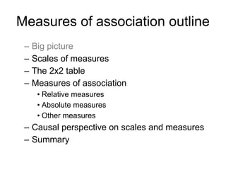
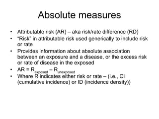
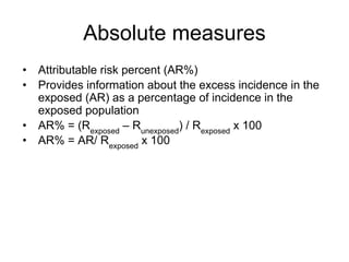
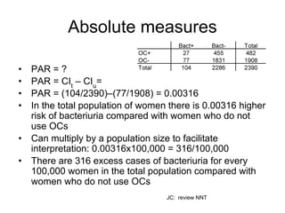
Absolute measures
• Alternative formulation for AR%
• Additional information/assumptions
– OR estimates risk/rate ratio
• AR% = [(OR – 1) / OR] x 100
• Alternative formula is a simple algebraic transformation
of original formula
– Dividing (Re
– Ru
) / Re
by Ru
– ((Re
/Ru
)-(Ru
/Ru
)) / (Re
/Ru
)
– (RR-1)/RR
– RR estimated by OR*
– *How well OR estimates risk or rate ratio depends on design of
case-control study and on how common disease is for
cumulative case-control

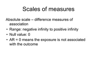
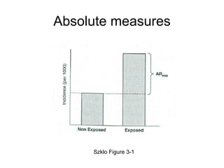
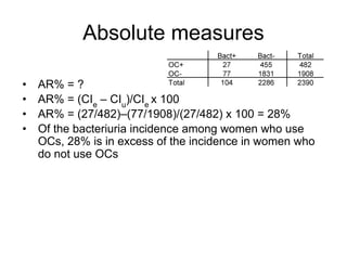
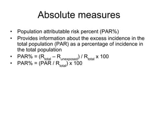
Absolute measures
• Alternative formulation for PAR%
– Prevalence of exposure in the total population can be estimated
as the proportion of non-diseased individuals exposed, or from
another source: Pe
– PAR% = [((Pe
)(OR-1)) / ((Pe
)(OR-1) + 1)] x 100
• Note Miettinen 1974 other formulation
– PAR% = AR% x (proportion exposed among diseased)
– Will provide a different estimate than formulation above

Absolute measures
• Derivation of alternative formula for PAR%
• Think of Rtotal
unexposed
• Weighted by the prevalence of the exposure:
– Rt
= (Re
)(Pe
) + (Ru
)(1-Pe
)
• Substitute into original equation
– PAR% = (Rt
– Ru
)/ Rt
– PAR% = ((Re
)(Pe
) + (Ru
)(1-Pe
) – Ru
)/ (Re
)(Pe
) + (Ru
)(1-Pe
)
– PAR% = ((Re
)(Pe
) + (Ru
)-(Ru
Pe
) – Ru
)/ (Re
)(Pe
) + (Ru
)-(Ru
Pe
)

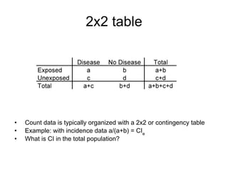
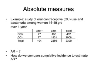
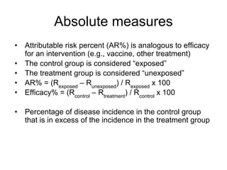
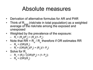
Absolute measures
• Divide numerator and denominator by Ru
– PAR% = ((Re
)(Pe
)/Ru
+ 1 - Pe
–1)/ (Re
)(Pe
)/Ru
+ 1-Pe
– PAR% = ((Re
)(Pe
)/Ru
- Pe
)/ (Re
)(Pe
)/Ru
- Pe
+ 1
– PAR% = (Pe
(Re
/Ru
- 1)/ Pe
(Re
/Ru
– 1) + 1
• Note that RR = Re
/ Ru
therefore if OR estimates RR
– PAR% = [(Pe
)(OR-1)] / [(Pe
)(OR-1) + 1]

Absolute measures
• Alternative formulation for AR, PAR
– Prevalence of exposure in the total population can be estimated
as the proportion of non-diseased individuals exposed, or from
an outside source: Pe
– Risk/rate for the total population can be estimated, usually from
an outside source: Rt
• Ru
= (Rt
) / ((OR)(Pe
) + (1- Pe
))
• Re
= (OR)(Ru
)
• AR = Re
-Ru
• PAR = Rt
-Ru

Absolute measures
• Derivation of alternative formulas for AR and PAR
• Think of Rtotal
unexposed
• Weighted by the prevalence of the exposure:
– Rt
= (Re
)(Pe
) + (Ru
)(1- Pe
)
• Note that RR = Re
/ Ru
therefore if OR estimates RR
– Re
= (OR)(Ru
)
– Rt
= (OR)(Ru
)(Pe
) + (Ru
)(1- Pe
)
• Solve for Ru
– Ru
= (Rt
) / ((OR)(Pe
) + (1- Pe
))
– Re
= (OR)(Ru
)

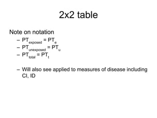
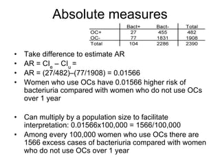
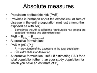
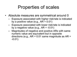
Absolute measures
• Formula review
– AR = Rexposed
– Runexposed
– AR% = [(Rexposed
– Runexposed
) / Rexposed
] x 100
– PAR = Rtotal
– Runexposed
– PAR = (AR)(Pe
)
– PAR% = [(Rtotal
– Runexposed
) / Rtotal
] x 100
– AR% = [(OR – 1) / OR] x 100
– PAR% = [((Pe
)(OR-1)) / ((Pe
)(OR-1) + 1)] x 100
– AR = (OR)(Ru
) - (Rt
/ [(OR)(Pe
) + (1- Pe
)])
– PAR = Rt
- [(Rt
)/ ((OR)(Pe
) + (1- Pe
))]

Properties of scales
• Absolute measures are symmetrical around 0
– Exposure associated with higher risk/rate is indicated
by a positive value (e.g., AR = 0.01)
– Exposure associated with lower risk/rate is indicated
by a negative value (e.g., AR = -0.01)
– Magnitudes of negative and positive ARs with same
numeric value are equivalent but in opposite
directions (e.g., AR = 0.01 same magnitude as AR =
-0.01)

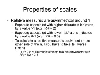
• Relative measures are asymmetrical around 1
– Exposure associated with higher risk/rate is indicated
by a value >1 (e.g., RR = 2)
– Exposure associated with lower risk/rate is indicated
by a value 0-1 (e.g., RR = 0.5)
– To calculate a relative measure’s equivalent on the
other side of the null you have to take its inverse
(1/RR)
• RR = 2 is of equivalent strength to a protective factor with
RR = 1/2 = 0. 5

• Relative measures – on arithmetic and log
scales

• Due to the asymmetry of relative measures
– Log-transformed (natural log) axes are often used to
graphically present relative measures
– Variances of relative measures are calculated on the
log scale, and any calculations based on the variance
(e.g., confidence intervals) are completed on the log
scale before returning to the relative measure scale

Variance estimates
• Approximate variance estimates for measures of
association (some are in Szklo appendix A)
• Variance of:
– ln(IDR) = (1/a) + (1/b)
– ln(CIR) = (b / a(a+b)) + (d / c(c+d))
– ln(OR) = (1/a) + (1/b) + (1/c) + (1/d)
• Small cells inflate variance

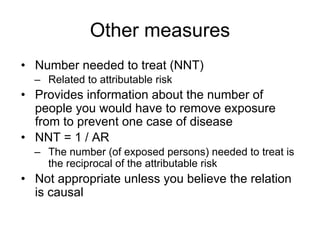
Other measures
• Number needed to treat (NNT)
– Related to attributable risk
• Provides information about the number of
people you would have to remove exposure
from to prevent one case of disease
• NNT = 1 / AR
– The number (of exposed persons) needed to treat is
the reciprocal of the attributable risk
• Not appropriate unless you believe the relation
is causal

Other measures
• Example of OCs and bacteriuria
• AR = 0.01566
• NNT = 1/AR = 1/0.01566 = 64
• 64 OC users need to stop using OCs to eliminate one
case of bacteriuria

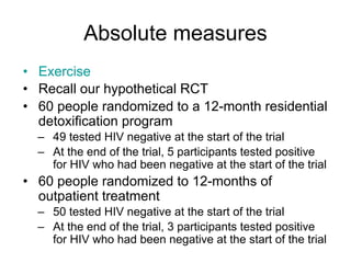
Absolute measures
• Exercise
• Recall our hypothetical RCT
• 60 people randomized to a 12-month residential
detoxification program
• 60 people randomized to 12-months of
outpatient treatment

Summary
• Measures of disease among groups with different
exposures are compared in observational epidemiology
• These comparisons are made with measures of
association between exposures and diseases
• Introduced to a variety of measures of association
broadly classified as relative or additive
Re
/Ru
Re
-Ru

Summary
• While the relative have been more commonly used, the
additive have been argued to be better for purposes of
identifying etiology and estimating public health impact
• Insights from two of the theoretical causal models
elucidate why this argument has been made, and
elucidate what relative and absolute measures estimate

Summary
Variety of terms used for measures of association
discussed today
• “Risk” often used generically to include rates (ID), risks
(CI) and even prevalence

Summary
Relative measures
• Cumulative incidence ratio (CIR)
• Incidence density ratio (IDR)
• Prevalence ratio (PR)
• Rate/risk ratio = Relative risk (RR)
• Odds ratio (OR)

Summary
Absolute measures
• Attributable risk (AR) = Risk/rate difference = Excess risk
• Population attributable risk (PAR) = Population risk/rate
difference
• Attributable risk percent (AR%) = Etiologic fraction =
Attributable proportion among the exposed
• Population attributable risk percent (PAR%) =
Attributable proportion in the total population

Summary
• Have only examined what are called “crude” measures
of association
– Compared exposed and unexposed populations without
considering other variables that may differ between the
populations
– Later in the course we will discuss how to deal analytically with
other variables that may be different between the exposed and
unexposed and that thus make the populations not
exchangeable (to be discussed in confounding)

Absolute measures
• Alternative formulation:
• PAR = (AR)(Pe
)
• Where does this come from?
• PAR = Rt
– Ru
• PAR = [(Pe
)Re
+ (1-Pe
)Ru
] - Ru
• PAR = (Pe
)Re
+ Ru
- (Pe
)Ru
- Ru
• PAR = (Pe
)Re
- (Pe
)Ru
• PAR = (Re
- Ru
)(Pe
)
• PAR = (AR)(Pe
)

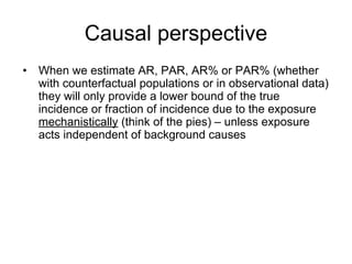
Causal perspective
• When we estimate AR, PAR, AR% or PAR% (whether
with counterfactual populations or in observational data)
they will only provide a lower bound of the true
incidence or fraction of incidence due to the exposure
mechanistically (think of the pies) – unless exposure
acts independent of background causes

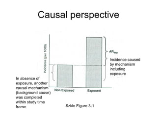
Causal perspective
Szklo Figure 3-1
Incidence caused
by mechanism
including
exposure
In absence of
exposure, another
causal mechanism
(background cause)
was completed
within study time
frame

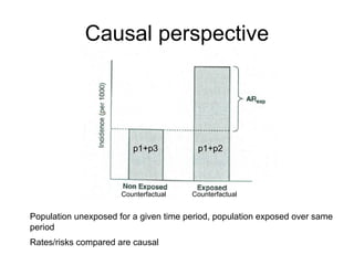
Causal perspective
Population unexposed for a given time period, population exposed over same
period
Rates/risks compared are causal
p1+p3 p1+p2
Counterfactual Counterfactual

Causal perspective
• Extreme example – mechanism including your exposure
causes disease 1 day earlier than would have occurred
otherwise from background causes
• In the exposed, your exposure mechanistically caused
100% of disease
• In your data the rate of disease appears the same in the
exposed and unexposed and you infer 0% of disease
caused by your exposure (ME3 p63, 297 for elaborated
discussion)
• Type 2 (slide 74) individuals (in this example 100% of
them) had disease caused by exposure when exposed,
but caused by another mechanism when not exposed
• Thus incidence due to specific causal mechanisms
cannot be estimated from epidemiologic data

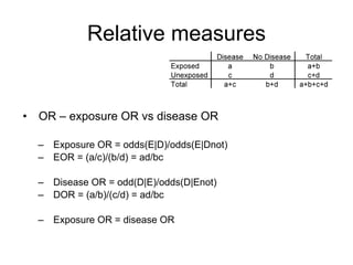
Relative measures
• OR – exposure OR vs disease OR
– Exposure OR = odds(E|D)/odds(E|Dnot)
– EOR = (a/c)/(b/d) = ad/bc
– Disease OR = odd(D|E)/odds(D|Enot)
– DOR = (a/b)/(c/d) = ad/bc
– Exposure OR = disease OR

2. ph250b.14 measures of association 1

Related slideshows

More Related Content

2. ph250b.14 measures of association 1