2011 IEEE International Conference on Control System, Computing and Engineering Power Optimization and Static Performance Investigation of an Island-mode Doubly-Fed Induction Generator (DFIG) Saad Mekhilef Department of Electrical Engineering University of Malaya Kuala Lumpur, Malaysia Saad@um.edu.my Omid Palizban Department of Electrical Engineering University of Malaya, Kuala Lumpur, Malaysia Omid.palizban@siswa.um.edu.my Abstract-- 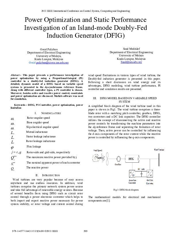This paper presents a performance investigation of power optimization by using a Proportional-Integral (PI) controller in a doubly-fed induction generator (DFIG). A detailed, dynamic model of a DFIG based on variable speed systems is presented in the dq-synchronous reference frame. Along with different controller types, a PI controller is chosen. Moreover, besides active and reactive power control, constraints and power optimization are discussed. Matlab software was used for simulation. wind speed fluctuations in various types of wind turbine, the Doubly-fed induction generator is presented in this paper. Following a short discussion on wind energy and its advantages, DFIG modeling, wind turbine performance, PI controller and simulation results are presented. Keywords-- DFIG, PI Controller, power optimization, power limitation A simplified block diagram of the wind turbine used in this paper is shown in Fig1. The wind turbine comprises a threeblade rotor with a matching pitch controller, gearbox, DFIG, two converters and a DC link capacitor. The DFIG controller utilizes the concept of disconnecting the active and reactive power controls by transforming the machine parameters into the dq-reference frame and separating the formation of rotor voltage. Then, active power can be controlled by influencing the d-axis components of the rotor current while the reactive power is controlled by influencing the q-axis components. I. ω ω ω L L L r b s m s r ϕ NOMENCLATURE Rotor angular speed Base angular speed Slip electrical angular speed Mutual inductance Stator leakage inductance DFIG MODEL BASED ON VARIABLE SPEED SYSTEM Rotor leakage inductance Flux linkage j = r, g max Q Rotor-side and grid-side, respectively The maximum reactive power provided by j j max S Q III. The nominal apparent power of each converter c The reactive power p II. INTRODUCTION Wind turbines are very popular because of easy access anywhere and use endless resources. In addition, wind turbines comprise the primary network system power source and take full advantage of renewable energy sources. Because of several benefits from using DFIG such as circuit rotor control through a power electronic converter which helps to both import and export reactive power necessary for power system stability, or rotor voltage and current control during 978-1-4577-1642-3/11/$26.00 ©2011 IEEE Fig.1: DFIG block diagram The mathematical models for electrical and mechanical components are[1]: 399 2011 IEEE International Conference on Control System, Computing and Engineering Fig.2 DFIG wind turbine simulation in Matlab Fig.2 shows the DFIG simulation done with the mentioned formulas and values from Table 1. A. Doubly-fed induction generator ∂ϕ 1 ω ∂t b 1 ∂ϕ ω ∂t b ∂ϕ 1 ω ω qs dr ∂t b ∂ϕ 1 ds b ∂t dr = R i + ω ϕ +V S dc e ds B. Rotor-side converter controller The rotor-side converter controller simulated in Matlab consists of four internal PI controllers (Fig.3). The two PI controllers are for active power (PI1 & PI2) and the others for reactive power (PI3& PI4)[2]. ds = V qs + R s i qs − ω eϕ ds = V dr + Rr idr + ω s ϕ dr = V qr + R r i qr + ω s ϕ dr (1) In addition: ϕ ϕ ϕ ϕ ds = −(Ls + Lm )i ds − Lm i dr dr = −(Lr + Lm )i dr − Lm ids qs = − (L s + L m )i qs − L m i qr qr = −(Lr + Lm )i qs − Lm i qs (2) Fig.3: Rotor side converter controller Using the general supposition of neglecting stator flux transients, the transfer function from the rotor voltage to the rotor current is approximated as: The electrical active and reactive power delivered by the stator is calculates as[2]: P = V i +V i Q = V i +V i s ds ds qs qs s ds qs qs ds ⎡ ⎤ ⎥ ⎡ I dr (s) I qr (s) ⎤ ⎢ 1 1 ⎢ ⎥ ⎥ = ⎢ ⎢ ⎛ ⎞ ⎛ ⎞ s s ( ) ( ) ′ ′ V V qr ⎦ R + S⎜ L r ⎟ R + S⎜ Lr ⎟ ⎥ ⎣ dr ⎢ r ⎜ ⎟ r ⎜ ⎟⎥ ⎝ ωb ⎠ ⎝ ωb ⎠⎦ ⎣ (3) Table 1: DFIG parameters & maximum operating limit of VCS (Pu) [1] [3] R R L L L S s r s r m max Cut-in wind speed Cut-out wind speed T T 0.0092 0.0076 0.19 0.0792 4.5926 0.3 5 25 (4) Moreover, the relation between rotor current, reactive and active power is calculated by: ⎡ Pt (s) Qr (s) ⎤ ⎡ S Lr ⎤ ⎢ ⎥ = ⎢Rˆ r + S Lˆ r Rr + ⎥ ωb ⎦ ⎣ I dr (s) I qr (s) ⎦ ⎣ T Where: 400 T (5) 2011 IEEE International Conference on Control System, Computing and Engineering ⎡⎛ ⎞⎤ − 1 ⎞⎛ = ⎢⎜ ωs ⎟⎜ Rr ⎟⎥ ⎜ ⎟ ⎜ ⎢⎣⎝ ωs ⎠⎝ ωb ⎟⎠⎥⎦ Rˆ r D. DC-link dynamic model and its controller The capacitor in the DC-link is an energy storage device. Neglecting losses, the time derivative of this capacitor’s energy depends on the difference in power delivered to the and the power provided by the DFIG rotor grid filter g (6) ⎡⎛ ω − 1 ⎞⎛ L ⎞⎤ s r Lˆ r = ⎢⎢⎜⎜⎝ ω s ⎟⎟⎠⎜⎜⎝ ωb ⎟⎟⎠⎥⎥ ⎦ ⎣ P circuit Therefore, the following formulas are obtained: P ≈ −P ω r s r , which can be expressed as: 2 1 C dc ∂ vdc = Pr − P g 2 ω b ∂t s P ⎛⎜⎝1−ω s ⎞⎟⎠ P (4) is used for PI2 and PI4 and (5) for PI1 and PI3. t≈ P (7) (8) s E. Reactive power controller The principle of the proposed voltage controller is to control voltage by adjusting the reactive power produced by the wind turbine, taking into consideration its operating state and limits. The reactive power necessary from an individual back-to-back voltage source converter when controlling the wind turbine is so significant that wind turbine operation limit does not exceed, and can be calculated as [4]: C. Grid-side converter controller Fig.4 shows a grid-side converter controller simulated by Matlab consisting of two internal PI controllers, PI5 and PI6. Q set j max ⎫ ⎧ Qj ⎪ ⎪ max = min ⎨Q , max Δ Q ⎬ max j pcc +Q ⎪ ⎪ Q r g ⎭ ⎩ Where P The input to the grid-side controller is the set of current values flowing to the network. The set of input current values is and Q maximum of set g g P set g and −1 Q set g set g ⎤ ⎥ ⎥ ⎦ reactive power. Therefore, the reactive j , which are operating-condition dependent, so the maximum available reactive power from every converter can be calculated by [3]: (8) Q max j = 2 ( S cmax ) − P − Q (10) 2 j p set g are the active and reactive power command set points. The value for P set g In addition, Fig.5 denotes is provided by the by (10) and (11) [4]: Table 2: Rotor and grid control gain parameters (Pu) [1][3] Controllers 0.0252 0.9995 0.7147 (− S highest reactive set points DC-link controller which determines active power flow and regulates DC-link voltage by driving it to a constant reference value [3]. PI1 & PI3 PI2 & PI4 PI5 & PI6 max max max ⎡ ;+ Q ⎤ − Q ⎢⎣ j j ⎥ ⎦ , as follows [3]: V d1⎤ ⎡⎢ P ⎥ V q1⎦ ⎢⎣Q Q power available from a single converter lies within the limits set ⎡ set ⎤ ⎡ V q1 ⎥ ⎢iqg set = ⎢idg ⎥ ⎢−V ⎣ ⎦ ⎣ d1 Where P is total reactive power required to support the pcc voltage at the point of common coupling (PCC). The active and reactive power operating limits are shown in Figure 5, wherein a rotor-side or grid-side converter must not exceed its apparent power limit represented by the half cycle. It is assumed that at a specific time every converter delivers active power j , after which the converter can supply or absorb a Fig.4: Grid-side converter controller calculated by the active and reactive power commands ΔQ (9) 10.4832 20 7.1515 401 Q max c set r max ≤ Pj ≤ Sc and Q ). Thus, the set g can be calculated 2011 IEEE International Conference on Control System, Computing and Engineering Fig.6 shows the stator reactive power control side simulated by Matlab. The upper circuit section does not have any effect on the reactive power set point. Therefore, the duty of this circuit control part is to create an interval limitation for reactive power. The bottom part of the figure represents voltage comparison and determining output reactive power. Fig.7: Output power based on different values of β Fig.8 shows overall conclusions regarding limitation and optimization. Fig.6: Active and reactive power operating limits As noted above, the stator output active and reactive power is in direct relation with rotor voltage. IV. Fig.8: Wind turbine limitation and optimization areas WIND TURBINE PRFORMANCE V. Wind turbine performance is divided into two parts: A. Power Optimization Optimization means producing maximum wind speed generation whenever wind speed, thus output power, is less than the nominal rate. To achieve this objective the pitch value (β ) is determined for a specific wind speed, thus maximizing the coefficient power value. The following equations show the power extracted by the blades: 1 3 (11) Po = 2 .ρ. A.V .C p Where CP is: ⎡ ⎤ (1 + vo ) ⎢1 − ( vo ) 2 ⎥ v ⎢⎣ v ⎥⎦ Cp = 2 With increasing C p PI CONTROL Fig.9 shows a complete PI controller diagram, which includes three parts: Fig.9: PI controller block diagram A. Power limitation in PI controller The pitch angle is determined by considering different dimensions between nominal power and measured power values in the PI controller for pitch angle control to output power limitation. The most important issue in PI controller design is preventing saturation of integral parts because when wind speed is less than nominal speed, or limited pitch angle is achieved, the set point does not equal zero, so the integral answer will be large. Because of this, the PI controller is designed with an anti-wind-up property (12) the output power increases equally. B. Power Limitation When the generator output power or wind speed is higher than the nominal value, power limitation must be performed in the system. In order to exploit the effect of stall control for limitation output power in this area of performance, blade angle must be changed in the negative direction. Fig.7 shows the output power based on different values of β . B. Transition logic By using wind speed and power values we need to choose between two modes: 402 2011 IEEE International Conference on Control System, Computing and Engineering • invastigation was carried out over 24 hours and all results on the time axis show those 24 hours (a day). Limitation of power: The output power or wind speed must be less than these transition nominal values. Optimization of power: The output power or wind speed must be more than these transition nominal values. 3 Output Active (watt) & Reactive (var) power of wind turbine • C. Pitch angle change system In this part of the PI controller, a display system for blade angle is desired. The DC motor is the system stimulus. As mentioned before, the system is modeled considering blade angle variations. The angle setting β sp compares with actual amount of angle (β) and the difference in these values is multiplied by P coefficient where there is maximum value variation in blade angle. VI. wind s peed (m /s ) R e a c ti ve p o w e r 2 1 0 -1 WIND TURBINE RESULTS VII. CONCLUSION In this paper, an induction generator simulation is presented by investigating equations related to DFIG. Then, directed control of the active and reactive power, as well as an investigation of wind turbine performance static were accomplished by using a PI controller, Rotor-side convertor, grid-side convertor and a DC link with a capacitor. In addition, by using a pitch angel controller, optimization and limitation zones are considered in wind turbine power generation, which are all clear on the curves related to the wind turbine output power. Reference: 20 [1] 10 0 6 12 18 24 2. Time (Hour) Fig.10: Wind speed variations over 24 hours 1.4 3. 1.2 1 4. Power (Pu) Ac ti ve p o w e r Fig.12: The output active and reactive power in DFIG 30 0.8 0.6 0.4 0.2 0 4 -2 The main issue with wind turbines is maximum operation limit in the voltage source converter (VSC) controller, of which values are defined in Table 1. As noted, the cut-in wind speed limitation for power generation is 5m/s and cut-off wind limitation is 25m/s. Fig.10 and 11 show the numerous wind speed variations investigated throughout a day and the results of the wind turbine power generating limitations, respectively. In this curve, the producing power is zero while the wind speed is less than 5m/s or more than 25m/s. 0 x 10 0 5 10 15 Wind Speed (m/s) 20 25 30 Fig.11: Optimization and limitation area results in Matlab The output active and reactive power from the doubly-fed induction generator is the same as in Fig.12. This 403 Hee-Sang Ko, G.-G.Y., and Won-Pyo Hong, Active Use of DFIG-Based Variable-Speed Wind-Turbine for Voltage Control in Power System Operation. Journal of Electrical Engineering & Technology, 2008. 3: p. 2. Hee-Sang Koa, Gi-Gab Yoonb, Nam-Ho Kyunga,Won-Pyo Hongc, Modeling and control of DFIG-based variable-speed wind-turbineElectric Power Systems Research, 2008. 78: p. 1841-1849. Ko, H.S., G.G. Yoon, and W.P. Hong, Active use of DFIG-based variable-speed wind-turbine for voltage regulation at a remote location. Power Systems, IEEE Transactions on, 2007. 22(4): p. 1916-1925. Ko, H.S., et al., Modeling and control of DFIG-based variable-speed wind-turbine. Electric Power Systems Research, 2008. 78(11): p. 1841-1849.