Experimentsin Fluids 17 (i994) 307 314 © Springer-Verlag1994 Stochastic estimation and proper orthogonal decomposition: Complementary techniques for identifying structure J. P. Bonnet, D. R. Cole, J. Delville, M. N. Glauser, L. S. Ukeiley 3o7 Abstract The Proper Orthogonal Decomposition (POD) as introduced by Lumley and the Linear Stochastic Estimation (LSE) as introduced by Adrian are used to identify structure in the axisymmetric jet shear layer and the 2-D mixing layer. In this paper we will briefly discuss the application of each method, then focus on a novel technique which employs the strengths of each. This complementary technique consists of projecting the estimated velocity field obtained from application of LSE onto the POD eigenfunctions to obtain estimated random coefficients. These estimated random coefficients are then used in conjunction with the POD eigenfunctions to reconstruct the estimated random velocity field. A qualitative comparison between the first POD mode representation of the estimated random velocity field and that obtained utilizing the original measured field indicates that the two are remarkably similar, in both flows. In order to quantitatively assess the technique, the root mean square (RMS) velocities are computed from the estimated and original velocity fields and comparisons made. In both flows the RMS velocities captured using the first POD mode of the estimated field are very close to those obtained from the first POD mode of the unestimated original field. These results show that the complementary technique, which combines LSE and POD, allows one to obtain time dependent information from the POD while greatly reducing the amount of instantaneous data required. Hence, it may not be necessary to measure the instantaneous velocity field at all points in space simultaneously to obtain the phase of the structures, but only at a few select spatial positions. Moreover, this type of an approach can possibly be used to verify or check low dimensional dynamical systems models for the POD coefficients (for the first POD mode) which are currently being developed for both of these flows. 1 Introduction In order to perform the projection required to obtain the time dependent random coefficients (the building blocks of the turbulent flow) from the Proper Orthogonal Decomposition (POD), it is necessary to have knowledge of the flow field at all points in space simultaneously. From an experimental point of view this requires that the flow domain be measured simultaneously on a sufficient spatial grid so as to minimize the effects of spatial aliasing as discussed by Glauser and George [12]. This is extremely difficult and can require hundreds of hot wire probes or full field measurement techniques which, as of yet, do not provide the necessary capability at high Reynolds number. The spatial two-point velocity correlation tensor on the other hand, a statistical quantity, can be obtained on a sufficient spatial grid with as few as two hot wire probes. In this paper a technique is proposed which uses the spatially resolved statistical quantity, the two-point correlation tensor, in conjunction with the instantaneous information at only a few select points, to obtain estimates of the time dependent random coefficients. The complementary technique is composed of three main steps. First, the eigenfunctions and eigenvalues are obtained from direct application of the POD to the two-point spectral tensor in both flows (see for example Glauser et al. [13], [14] and [15] for the jet and Delville et al. [7], [9] and [lo] for the plane mixing layer). Second, the Linear Stochastic Estimation (LSE) [1] is applied to the cross-correlation tensor and multipoint estimates of the random vector field are computed as described by Cole et al. [5]. Third, the estimated velocity field obtained from step two is projected onto the eigenfunctions obtained from step one to obtain the estimated random coefficients. The estimated random coefficients are then used in conjunction with the POD eigenfunctions to reconstruct the random velocity field. In this study, Received: 27 September~Accepted: 2 May 1994 only time and the strongly inhomogeneous direction are examined for both flows. The authors recognize that coherent strucJ. P. Bonnet, J. Delville Centre D'Etudes Aerodynamiques et Thermiques, F-86ooo Poitiers, France tures are 3 dimensional in nature and that it can be quite misleading to extract information from 2 dimensional slices. HowD. R. Cole, M. N. Glauser, L. S. Ukeiley ever, in this paper the thrust is not to extract physics, but to Department of Mechanical and Aeronautical Engineering, demonstrate the usefulness of the complementary technique in Clarkson University, Potsdam, NY 13699, USA 2 flows where the instantaneous velocities are available simulCorrespondence to: M. N. Glauser taneously at a cross section in the flow on a sufficient spatial grid. This allows for comparisons to be made between the reconstructed The authors wish to thank DRET Grant # 9o/171, the French Embassy measured velocity field obtained from direct application of the POD Chateaubriand Fellowship (CIES)program for L. Ukeiley,NASA/LewisGSRP to that obtained from application of the complementary technique. for D. Cole, NASA/AmesDryden, NASA/Langleyand NSF/CNRSthrough the It should be emphasised that the complementary technique allows international travel grants program for funding various portions of this for unique applications of the POD, in particular, to real 3D work. simultaneously at each x2 location. The numerical instantaneous fidds. In this section, POD and LSE are briefly reviewed and the complementary technique introduced. approximations of Eq. 2 and 4 involves replacing the integrals by an appropriate quadrature rule (in this study a trapezoidal rule) as detailed by Glauser et al. [13]. 1.1 POt) theo~ 308 The POD was first proposed by Lumley [18] in 1967, as a mathematically unbiased technique for extracting structures from turbulent flows. Lumley proposed that the coherent structure be that structure which has the largest mean square projection on the velocity field. This maximization leads to an integral eigenvalue problem which has as its kernel the cross-correlation tensor, Rij(~, U, t, t'). This technique has recently become more popular with the development of more powerful computers and advanced data acquisition equipment. For example, Moin and Moser [20] applied the POD to the full correlation tensor which was generated numerically from simulations of turbulent channel flow and Ukeiley et al. [23] applied it to an experimental data base obtained in the complex flowfield downstream of a lobed mixer. For a recent comprehensive review of the POD see Berkooz et al. [4]. The POD reduces to the harmonic orthogonal decomposition in time since both flows are stationary, hence the eigenfunctions used in time are Fourier Modes. Only the radial direction (r) in the jet and the cross-stream direction (y) in the mixing layer, which are both strongly inhomogeneous in their respective flows, are examined with the POD. For the following analysis a coordinate system of xl, x 2 and x3 is used. For the jet; xi = z the streamwise direction, Xa= r, the radial direction and x3 = 0, the azimuthal direction. For the mixing layer; x~--x, the streamwise direction x2=y, the cross-stream direction and x3 = z, the spanwise direction. Given the afore-mentioned conditions, the spectral tensor may be defined by the following equation, t 0 0 So(xz, x2,fXl, X3)=~Rij(Xz ' x2,, r, xl,o x3o ) e-i2'q~ dz, (1) , Rij (x2, x2,, "c, xx,0 x 30 ) = u i (x2, t, x l0, x 30 ) uj (X2, t + Z, X~, X~). In the above equation, f denotes frequency, ~ is the separation in time and x~ and x ° represent the azimuthal and streamwise locations in the jet, and spanwise and streamwise locations in the mixing layer where the correlation tensors were measured. In this formulation, S0 becomes the kernel in the integral eigenvalue prbblem which is written as: where (z) The $'s and 2(")(f) are the frequency dependent eigenfunctions and eigenspectra respectively. Note that dx'2 = r' dr' for the jet and dy' for the mixing layer. The Fourier Transform of the velocity can be reconstructed in terms of the ~'s as; hi= (x2,f) = ~ a,,( f)l/I}'O(xz,f), (3) n=l where an(f) = 5f*i(x2, f ) ~ f~)(x2, f)dx2. In 1975, Adrian [1] proposed that stochastic estimation could be applied to unconditional correlation data. This method uses what Adrian calls a "conditional eddy". This eddy is a candidate structure used to detect, within certain limits, other structures of similar type. Stochastic estimation uses the conditional information specified about the flow at one or more locations in conjunction with its statistical properties to estimate the information at the remaining locations. Adrian [1] studied conditional flow structures in isotropic turbulence by computing estimates of the velocity u(x', t) given that the velocity at (x, t) assumes some specified value u(x, t). He found that this simple flow, when sampled in a statistical sense, shows the existence of organized structures. He used a second order stochastic estimation technique, but concluded that first order (linear) stochastic estimation (LSE) would have resulted in nearly identical estimates. This indicates that the second order term contributed little to the overall estimate. Tung and Adrian [2z] studied the influence of the third and fourth order terms on the estimate as well as the second order term. Their results confrmed the insignificance of the higher order terms on the overall estimate. Moin, Adrian and Kim [19] applied stochastic estimation, in order to approximate conditional vector fields, to a numerically simulated channel flow. One of their most interesting results, but only discussed briefly, was that they found good agreement between the LSE and Lumley's characteristic eddy. This was further examined by Moser [21] but comparisons were difficult because of the ambiguity in domain selection for the application of the POD (i.e., different subdomains in the boundary layer). For further discussion on the Stochastic Estimation theory see Adrian and Moin [z] and Guezennec [17]. As discussed above, Tung and Adrian [z2] have shown that linear stochastic estimation produces reasonable qualitative estimates and little is to be gained by using second order or higher. Linear stochastic estimation yields an estimate ~i(x') = Ao(x')uj(x) ~s~j(x~, x;,f, x °, x~) ~,~")(xl, f, 4 , x ° )dx; _ ; ( , ) ( f ) O,(,) (x2,f,x,,x3). o o 1.2 Stochastic estimation theory (4) So(x2, x'2,f, x°,, x~) is obtained from the experimental measurements in both flows and used in conjunction with Eq. z to extract the eigenvalues and eigenfunctions. Note: To compute a~(f) using Eq. 4, ~i(x2,f) must be available (5) with &k computed from, uj(x) Uk(X) aik(X') = Uj(X)Ui(X') (6) where uj(x)Uk(X) and uj(x)ui(x') are the Reynolds stress and two-point correlation tensors respectively. For the u, v jet and mixing layer data (u = ul and v = Uz), the matrices that result from the expansion of Eq. 6 for a two probe estimate are: First System: ry -~r , , Ur~Vr~ v2, l U~2Ur~ IXr~!Yr~ Lv~2Ur~Vrz!/rt I (7) Second System: using the original measured instantaneous velocity data as given by the inverse Fourier transform of Eq. 3. A flow chart which compares the steps involved in the complementary technique to those for a direct application is presented in Fig. 1. I;r U" UFUUrq F4 V2rl Vr~Zr2 ~ U,'zVr t bi2rz bT, ~]r21]r~ Vrzbir2 ~r2 I jlA r ,/ (8) 2 Experiments L~M U~s/ where rl and r2 refer to reference probes 1 and a respectively, and p refers to the probe number. It should be noted, that for these systems of equations, only the two-point space-time correlation data is utilized. These systems are not a function of the condition being investigated. The estimated velocity components for the two probe reference case can then be found from the expansion of Eq. 5, ~ rl rl r2 big __ -- AilpUCr~ + AlzpVCrl -[- A r21]pucr2+ AlzpVCr2 (9) and " -. . . . Y2 Y2 • Vp -A2ipUCr, + A22pVCr,+ A21pUCr~ + A22pVCT~ (10) It is in these estimated velocity equations that the condition selected plays a role (i.e., through u G, u % v G and vG). A single probe estimate is obtained by merely setting all terms containing r2 = o. Without much trouble this system can easily be expanded to include estimates for all of the probes. This should result in the estimated velocities being exactly the same as the actual velocities. This property can then be used as a check. In this paper it is not the intent of the authors to discuss what number of probes or their respective positions are the most appropriate to obtain the best estimate of the velocity field. These issues are discussed in Cole et al. [5] for the jet and in Delvile et al. [8] for the mixing layer. 1.3 Complementary technique The complementary technique utilizes the POD eigenfunctions, as described in the POD Theory section, and the LSE of the velocity field, as described in the Stochastic Estimation Theory section, to obtain estimates of the random coefficients from which the velocity field can be reconstructed. Mathematically the stochastic estimates of the random coefficients are calculated from ann est( f ) = S~ St(Xz,f ) ~P}")*(X2,f ) d x , (11) where fi~St(xa,f) is either a single or multipoint (in this study, 2 point) linear stochastic estimate of the velocity field (from the time Fourier Transform of Eq. 9 and 10) and 0~")*(x2,f) is obtained from the original POD eigenvalue problem. Note the similarity to Eq. 4, here however the actual velocity field is replaced by that estimated from the 2 point linear stochastic estimate. The estimated u or v velocity can then be reproduced in Fourier space by ^ est (xz, f ) ui = anest(f)Oi (~)(x2'f) The jet shear layer and 2-D mixing layer experiments, which are used in this study, are flows where the instantaneous velocities are available simultaneously at a cross section in the flow on a sufficient spatial grid. This allows for comparisons to be made between the reconstructed measured velocity field obtained from direct application of the POD to that obtained from application of the complementary technique. Each of these experiments is briefly described below. 2.1 Jet The experiment conducted to obtain the data in the axisymmetric jet was first reported by Glauser and George [13] and Glauser et al. [14]. The jet had an exit diameter (V) of 0.098 m with a centerline exit velocity of 2o m/s. The Reynolds number based on exit diameter was 11o,ooo with a 0.35% turbulence intensity in the core region. The data was collected by two rakes each containing 4 "X" wires. The rakes were placed 3 jet diameters downstream. In the original experiment the rakes were traversed through 25 azimuthal locations, however in this study only the azimuthal position of 0 = o is examined. The hot wires were spaced by approximately lo.9 mm, making the total distance spanned 76.2 mm, which is approximately twice the vorticity thickness. The sensing wire used were 5 gm in diameter and had a sensing length ofl.2 ram. In order to achieve the ensemble averages necessary to calculate the correlation tensor 3oo blocks of lO24 samples were collected. The data was low pass filtered at 800 Hz while being sampled at 2000 Hz. The data acquisition system was based around a 15 bit, 16 channel A/D converter with simultaneous sample and hold capability. 2.2 Mixing layer The experiment to obtain data in the subsonic plane mixing layer was performed at CEAT/LEA in Poitiers, France. The subsonic turbulent plane mixing layer had a high speed velocity of 42.8 m/s and a low speed velocity equal to 25.2 m/s. All the measurements were taken at 6oo mm downstream of the trailing edge of the splitting plate, where the vorticity thickness was 27.6 mm. A rake of 12 equally spaced "X" wires was utilized to obtain the data. The probes were placed symmetrically about the mixing layer axis and the separation between them was 6 mm. The diameter of the wires was 2.5 gm with a sensing length of 0.5 mm. The data was simultaneously sampled at lO kHz using constant temperature anemometers built from a TSI 175o. For further information the reader is referred to Delville et al. [7]. (12) n=l and then inverse transformed to obtain u~St(x 2, t). Comparisons are then made, for both flows, between the reconstructed estimated velocity field as described by Eq. lZ and those obtained 3 Results As was discussed in the introduction, in this study only time and the strongly inhomogeneous direction are examined in both 309 Complementary Teeh. Direct Method Measure Ui(~,,t) at all positions in space simultaneaously . . . . . . . . . . . . . . . . . . . . . . . . . . . . . . . . . . . . . . M_easuse~J . . . . . . . . . . . . . . Note: requires a minimum of two probes Note: requires a significant amount of probes J Compute Rij and extract POD eigenmodes 31o Extract POD eigenmodes I I Use LSE to obtain estimate of Ui~,t) at all positions in space Project Ui(x,t) onto POD eigenfunctions to compute the random coefficients I Project estimated Ui(x,t) onto POD eigenfunctions to obtain an estimate of the random coefficients t Rebuild original field at all space location t I Rebnild estimated field at all space locations I I 0 90 ~-~ • ~ . . ~ ~ K ' ~ . . ~ , , . _ _ ~ .-'---T'r'C'~ ~"-YZ'~'~--~,¢'/I///,,,"If~ 0.13 ~""-:: -~~ ..... "~'-"~ " ............... :'~.~- a. . . . . . . . . . . . . . . . . * ...... ~ ~ , , " ....... 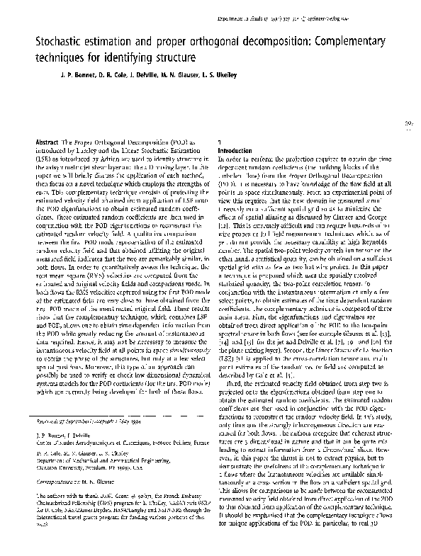""'""~ ""~-''"~ ,~_;" Fig. 1. Flow chart showing comparison between complementary technique and direct application "-,,w,+~ .......... Fig. 2. Instantaneous velocity vector plots of the jet seen in a frame of reference moving at uc= 12 m/s flows. More complete analysis of these data bases, including multi-dimensional analysis, have been reported by Glauser et al. [15] and Delville et al. [8] for the jet and mixing layer respectively. Vector plots are used here to qualitatively examine the flow fields. Figure 2 presents an original measured velocity field for the axisymmetric jet shear layer at one azimuthal position seen in a frame of reference moving at 12 m/s. This record contains 15o time steps, which corresponds to o.073 sec. Figure 6 presents an original measured velocity field for the plane mixing layer at one spanwise location seen moving in a reference frame of 33.7 m/s. In this case there are also 15o time steps, but the corresponding time is only o.o15 sec. Note that, in the times selected for the respective flows, several large scale motions are observed. Vector plots of the contribution from the first POD mode for the jet shear layer and the plane mixing layer are shown in Figs. 3 and 7 respectively, using the original measured instantaneous velocity field in each projection. These are obtained by direct application of the inverse Fourier transform of Eq. 3. For both flows, the first mode exhibits most of the large scale features observed in the original velocity fields (Figs. 2 and 6 for the jet and mixing layer respectively) although they do not have the same spatial extent in the visualization• Although not presented here, the spatial information fills in when more modes are retained as shown by Glauser et al. [15] and Ukeiley et al. [24] for the jet and Delville et al. [9] for the mixing layer. Figures 4 and 8 show two-point linear stochastic estimates of the original measured velocity field for the jet mixing layer and the plane mixing layer, respectively. In these cases instantaneous information at two points is utilized as the condition from which the remaining information is estimated. The probes which supply the condition are equally spaced on either side of the centerline for both flows• Compare Figs. 4 and 8 to Figs. 2 and 6, respectively• Note how much of the structure observed in the visualizations of the original measured signals is contained in these two-point estimates and, in particular, how the phase information is preserved. The structures Fig. 3. A ~ POD mode reconstruction of the jet 311 Fig. 4. StochasticEstimated field of the jet using the wires indicated by the arrows as reference I T T F ~ I L I . ~ . . I . ~ 2 ~ £ ~ 2 ~ ' ~ . ~ . ~ ...... ; ~ ~ ~ ; ~ 2 ~ ; ~ 1 ~ T ~ : ~ 2 ~ Fig. 5. Complementarytechnique: A 1 POD mode reconstruction of the jet using the stochasticallyestimated field .. ,4~ ;'1 18 Fig. 6. Instantaneous velocityvector plots of the mixing layer seen in a frame of reference moving at Uc=33m/s characteristics are slightly underpredicted. As would be expected, at the conditional probe positions, all of the features are captured. It is also seen that the estimates using the data taken in the plane mixing layer produce better defined structures. It was shown by Cole et al. [5] that a single point reconstruction for the jet shear layer is inadequate and that the best estimates occurred when the condition utilized information from both sides of the jet shear layer. It was found in the plane mixing layer, however, that when using a probe placed at the outer region of the shear layer, the large scale motions were fairly well represented as discussed by Delville et al. [8]. These differences can be attributed to the difference in integral length scale between the two flows. In Figs. 5 and 9 the results from the application of the complementary technique are presented for the jet mixing layer and the plane mixing layer, respectively. The estimated fields (Application of Eqs. n and 12 using the estimated data presented in Figs. 4 and 8), are projected onto eigenfunctions obtained from direct application of the POD. Reasonable estimates of the large scale structure are obtained, but only a small percentage of the original measured instantaneous data (25% for the iet and 17% for the mixing layer) has been usedK In fact, one sees that Figs. 5 and 9 compare quite well to Figs. 3 and 7 respectively, which were computed using the full measured instantaneous velocity field. It should be noted that more features are recovered away from the center of both the jet shear layer and the mixing layer from the first POD mode reconstruction of the estimated field than the estimated field contains itself. This can be seen by comparing Figs. 5 and 9 to Figs. 4 and 8 respectively. It is apparent that this effect is most dominant for the mixing layer. Evidently, the first POD eigenfunction, used in the projection, contains a significant amount of knowledge of the velocity field (in the averaged mean square sense) and hence provides the 22.'~22'" ' ................ !222! ........... ~2!~....... ! ! ! 2 ; ! 2 ! . : ! : : : 2 ! ~ .............. 5'-2!!:!~'.22................ : ~ ' 2 Y ' Fig. 7. A 1 POD mode reconstruction of the mixing layer ~::'~: :: : : : : : : : : : : : : : : : : : : : : : ====================================== . ~ _ , : . . ~ . ~ - . . . ~ 1 .- . .,~ "-',l~r Fig. 8. Stochastic Estimated field of the mixing layer using the wires indicated by the arrows as reference -- , . . . . . . . . . . .... =========================================================== ......... , ........... :-:x ....... ~::::: .......... :::; ...... ......................................... -",," .... : ........ ::2..... ' .......... ~.............. ;;:to: ............ " .......... ~. . . . . . Fig. 9. Complementary technique: A 1 POD mode reconstruction of the mixing layer using the stochastically estimated field additional information. It has been observed by Ukeiley et al. [24] that more spatial information is filled in when additional POD modes are included. They also note that the 3 POD mode representations of the estimated fields do not compare as well to the 3 POD mode representation of the original measured field when compared to the 1 POD representations (i.e., the results differ more as additional POD modes are used). This could be interpreted as a surprising result, but this is not unexpected since the sum of all the terms in Eq. n will result in the estimated field being recovered and not the original measured field. These results are summed up quantitatively in Figs. lo and 11 for the jet shear layer and plane mixing layer respectively. These figures present comparisons between the original measured and estimated streamwise RMS velocities, and 1 POD mode representations of each of them. What is seen in Fig. lo, for the jet shear layer, and in Fig. 11, for the plane shear layer is that the complementary technique captures almost as much of the RMS streamwise velocity in a single POD mode, as the direct application of the POD to the original measured velocity. It is also evident from Fig. al, as was observed in the instantaneous plots and discussed in the previous paragraph, that the complementary technique does a significantly better job at predicting the flow characteristics away from the center of the plane mixing layer than the LSE alone. Recently, Ewing [11] has examined the question of aliasing for the complementary technique. Although not shown, the eigenspectra for the first mode computed from the estimated coefficients 0.20 L i i I i i J • Original - - -~ S t o c h a s t i c Est. ..... 1 POD m o d e + - - - - - + Comp. Tech, . o.15 I 0.10 l "= / / , 0.05 ' p//.¢ \ \ ~ > ,S/ • / 13" 0 o., I & , ' o's riD ---..-- Fig. lo. RMS comparisons for the jet 016 01.7 018 0.9 0.100 ~~ Original /k ] . . . . ~ StochasticE s t . / I ..... 1 POD mode / ~----.Comp.~,,~ 0.075 t l q f \1 ff 0.050 " \ \\ 'L , ,/// / 15': , l/ 0.025 0-1.2 --' - -u-,-0.8 f j -0[4 0 y/&~ I I 0.4 0.8 1.2 = experimentalists to avoid using Taylor's "Frozen Field" hypothesis in the streamwise direction. At the present time, the correlation tensor is typically obtained at one downstream location and Taylor's hypothesis used to infer the streamwise dependence of the correlation tensor. This procedure has been implemented mainly to avoid flow blockage affects of the upstream rakes of hot wires on the downstream measurements. The new approach involves measuring apriori, the correlation tensor at several downstream positions independently. The experiment is then repeated with a minimal amount of strategically placed probes, all sampled simultaneously, at each of the streamwise locations where the correlation tensor has been measured. The LSE can then be implemented using this instantaneous data, in conjunction with the well resolved correlation measurements available at each downstream location, to obtain an estimate of the entire spatial and temporal velocity field. Finally, an estimate of the streamwise evolution of the correlation tensor can be computed from the estimated velocity feld. The streamwise evolution of the POD eigenfunction can then be extracted, hence avoiding the use of Taylor's hypothesis. Fig. 11. RMS comparisons for the mixing layer References (2~st(f) =a~St(f)a~ est (f)) are very close to the original eigenspectra in both flows. This indicates that the effects of aliasing are minimal for the two applications presented here. 4 Conclusions and future work The POD and LSE have been combined in a novel fashion utilizing the global nature of the POD and the local nature of the LSE. The two-point LSE estimated instantaneous field is projected onto the eigenfunctions obtained from the direct application of POD and a 1 POD mode representation computed for both the jet shear layer and plane mixing layer. These results are remarkably similar to a 1 POD mode representation of the original measured instantaneous field. Hence, the complementary technique retains the phase information of the POD modes, from the instantaneous signal obtained at a "few" select spatial locations and knowledge of the instantaneous field at all spatial positions is not necessarily required. RMS velocity plots, which are used to quantify the effectiveness of the complementary technique, confirm this as well. They show that a 1 POD mode representation of the RMS estimated field is very close to that obtained from a 1 POD mode representation of the RMS original measured field. In this work the complementary technique was used to obtain estimates of the random coefficients in the strongly inhomogeneous directions for both the jet shear layer and plane mixing layer. In the future, the technique can be used in a similar manner as described above to obtain estimates of the random coefficients in the remaining directions as well. Hence this type of an approach can possibly be used to verify or check low dimensional dynamical systems models for the POD coefficients (for the first POD mode) which have been developed in the boundary layer by Aubry et al. [3], in the jet by Glauser et al. [16] and which are currently under development for the plane mixing layer by the authors. An additional useful application of the LSE and POD in tandem holds forth the possiblity of allowing 1. AdrianRJ (1975) On the role ofconditionalaveragesin turbulence theory. Turbulence in Liquids. Science Press, Princeton, NJ, pp 323-332 2. AdrianRJ; Moin P (1988) Stochastic estimation of organized turbulent structure: Homogeneous Shear Flow. J Fluid Mech 19o: 531-559 3. Aubry N; Holmes P; LumleyJL; Stone E (1988) The dynamics of coherent structure in the wail region of a turbulent boundary layer. J Fluid Mech 192:115-173 4. Berknoz G; Holmes P; LumleyJL (1993) The proper orthogonal decomposition in the analysis of turbulent flows. Annu Rev Fluid Mech. 25:539-575 5. ColeDR; GlauserMN; GuezennecYG (1992) An application of stochastic estimation to the jet mixing layer. Physics of Fluids A, 4(1): 192-194. 6. Cole DR; UkeileyLS; Glauser MN (1991) A comparison of coherent structure detection techniques in the axisymmetric jet mixing layer. Bulletin of the American Physical Society,36(lO) 7. DelviUel; Bellin S; Bonnet lP (1989) Use of the proper orthogonal decomposition in a plane turbulent mixing layer, in Turbulence and Coherent Structures. (O Metals and M Leiseur eds.) Kluwer Academic Press, The Netherlands, pp 75 90 8. DelvilleJ; Vincendeau E; UkeileyL; Garem JH; Bonnet JP (1993) Etude Exp~rimentale de la Structure d'une Couche de M61ange Plane Turbulente en Fluide Incompressible. Application de la D&omposition Orthogonale aux Valeurs Propres. Convention DRET 9o-171 Rapport F~aal. 9- DelvilleJ (1993) Characterization of the organization in shear layers via the proper orthogonal decomposition, in Eddy Structure Identification in Free Turbulent Shear Flows. (JP Bonnet and MN Glauser eds.), Kluwer Academic Press, The Netherlands, pp. 225-238. lo. DelvilleJ; UkeileyL (1993) Vectorial proper orthogonal decomposition, including spanwise dependency,in a plane fully turbulent mixing Layer. Proceedings, Ninth Symposium on Turbulent Shear Flow, Kyoto, Japan, pp 10.3.1-10.3.611. EwingD (1994) Private Communication, Department of Mechanical and Aerospace Engineering, University at Buffalo/SUNY iz. Glauser Mark N; GeorgeWilliam K (1992) Application of Multipoint Measurements for Flow Characterization. Experimental Thermal and Fluid Science, 5:617-632 13. GlauserMN; Leib SJ; GeorgeWK (1987) Coherent Structures in the AxisymmetricJet Mixing Layer. Turbulent Shear Flows 5, Springer Verlag, pp 134-145 14. Glauser MN; GeorgeWK (1987) An orthogonal decomposition of the AxisymmetricJet Mixing Layer utilizing Cross-Wire Measurements. 313 15. 16. 17. 18. 314 19. Proceedings, Sixth Symposium on Turbulent Shear Flow, Toulouse, France, pp lO.1.1-1o.1.6. Glanser MN; Zheng X; George WK (1992) An analysis of the Turbulent Axisymmetric Jet Mixing Layer. In Review J Fluid Mech Glauser MN; Zheng X; Doering C (1992) A low dimensional description of the axisymmetric jet mixing layer utilizing the proper orthogonal decomposition. In review Physics of Fluids A Guezennec ¥G (1989) Stochastic estimation of coherent structures in turbulent boundary layers. Phys. Fluids A, 1(6): lO54-1o6o Lumley ]L (1967) The structure of inhomogeneous turbulent flows. Atm. Turb. and Radio Wave Prop. (Yaglom and Tatarsky eds.) Nauka, Moscow, pp 166-178 Moin P; Adrian RJ; Kim ] (1987) Stochastic estimation of organized structures in turbulent channel flow. Proceedings, Sixth Symposium on Turbulent shear flows, Toulouse, France, pp 16.9.1-16.9.8. 2o. Moin P; Moser RD (1989) Characteristic-Eddy decomposition of turbulence in a channel. ] Fluid Mech. zoo: 471-5o4 zx. Moser RD (1988) Statistical analysis of near-wall structures in turbulent channel flow. Proceedings, Symposium on Near Wall Turbulence, Dubrovnik, Yugoslavia, pp 45-62. z2. Tung TC; Adrian RI (198o) Higher-Order estimates of conditional eddies in isotropic turbulence. Phys Fluids 23: 1469-147o 23. Ukeiley L; Glauser M; Wick D (1993) Downstream evolution of proper orthogonal decomposition eigenfuncfions in a lobed mixer. AIAA Journal 31(8) 1392 1397 24. Ukeiley L; Cole D; Glauser M; (1993) An examination of the axisymmetric jet mixing layer coherent structure detection techniques, in Eddy Structure Identification in Free Turbulent Shear Flows. (JP Bonnet and MN Glauser eds.), Kluwer Academic Press, pp 325-336 lnnouncemen CALL FOR PAPERS Symposium on Flow Visualization and Image Processingof Multiphase Systems 1995 Fluid Engineering Division Summer Meeting (ASME/EALA Sixth International Conference on Laser Anemometry) American Society of Mechanical Engineers Hilton Head, South Carolina U.S.A. August 13-18, 1995 This symposium is sponsored by the Multiphase Flow Committee of the ASME Fluids Engineering Division. It will be a part of the ASME/EALASixth International Conference on Laser Anemometry under the auspicious of the ASME Fluids Engineering Division summer Meeting ('95 FEDSM). Flow visualization is an important experimental methodology which has been instrumental in promoting and establishing modern science and technology. It is, presently, extensively employed in various scientific and high-technology fields. With rapid advances in computer and image processing techniques, visualization science has become a dynamic multidisciplinary field of learning not only in the past and present but also in the future. Its applications cover practically all areas in science and technology. This symposium is intended for visualizing multiphase flows and obtaining quantitative information through image processing. Prospective contributors are requested to submit three copies of a 300 word abstract. The abstract should clearly state the method, results and indicates the name, address, phone number, and fax number of the corresponding author. Final acceptance of the papers will be based upon the review of the complete manuscript according to ASME standards. All accepted papers will be published in a symposium volume that will be available at the meeting. DEADLINES Submission of abstract to Symposium Chair: August 31, 1994 Notification of preliminary acceptance: October 14, 1994 Full-length papers due to Symposium Chair: November 28, 1994 Notification of final acceptance and sent mats: February 1o, 1995 Final typed mats due to Symposium Chair: April lo, 1995 Symposium Organizers: Wen-Jei Yang, Chair Dept. of Mech. Eng. & Appl. Mech. University of Michigan 215o G.G. Brown Bldg. Ann. Arbor, MI 481o9, U.S.A. F. Yamamoto Dept. of Mech. Eng. Fukui University Fukui 91o, Japan F. Mayinger Institut ffir Thermodynamik A Technische Universit~it Miinchen Postfach zoz4zo D-8o333 Miinchen, Germany Tel: (313) 764-991o Fax: (313) 747-317o Tel: o776-27-8534 Fax: 0776-27-8748 Tel: 49-89-ZLO5-3451 Fax: 49-89-ZlO5-2ooo