JOURNAL OF PLANKTON RESEARCH j VOLUME 30 j NUMBER 9 j PAGES 1041 – 1049 j 2008 FERNANDO VILLATE1*, GUILLERMO ARAVENA1, ARANTZA IRIARTE1 AND IBON URIARTE2 1 LABORATORY OF ECOLOGY, DEPARTMENT OF PLANT BIOLOGY AND ECOLOGY, FACULTY OF SCIENCE AND TECHNOLOGY, UNIVERSITY OF THE BASQUE COUNTRY, 644, 48008 BILBAO, SPAIN AND 2LABORATORY OF ECOLOGY, DEPARTMENT OF PLANT BIOLOGY AND ECOLOGY, FACULTY OF PHARMACY, UNIVERSITY OF PO BOX THE BASQUE COUNTRY, PASEO DE LA UNIVERSIDAD 7, 01006 VITORIA-GASTEIZ, SPAIN *CORRESPONDING AUTHOR: fernando.villate@ehu.es Received March 10, 2008; accepted in principle May 12, 2008; accepted for publication May 20, 2008; published online May 24, 2008 Corresponding editor: William Li The relationships between chlorophyll a concentration and environmental (climatic and associated hydrographical) factors were investigated in the estuary of Urdaibai (Bay of Biscay) in different salinity zones of the euhaline region, using time-series for the period 1997– 2006. Transfer function (TF) models were used on quarterly data (3 month mean values) to establish possible relationships between time-series. In the non-nutrient limited waters with salinities of 30 and 33 PSU, a chain of effects from the North Atlantic Oscillation (NAO) to chlorophyll a was established, where air temperature followed inversely the NAO index, water temperature followed air temperature and chlorophyll a followed water temperature. Each of the steps occurred with a lag of 0 (within the 3 month period); however, the effect from NAO to chlorophyll a showed a lag of 1 (a mean of 3 months delay). Consistent with this result, annual mean chlorophyll a biomass in the 30 and 33 PSU salinity zones showed a significant positive relationship with annual mean water temperature and a significant negative relationship with the 12 month mean NAO index from October of the previous year to September. In the 35 PSU salinity zone, no significant relationship between chlorophyll a and NAO or water temperature was observed. It is suggested that nutrient limitation distorts the effect of temperature on phytoplankton biomass enhancement in the outer estuary (35 PSU salinity zone). I N T RO D U C T I O N It is well known that meteorological factors affect phytoplankton dynamics (Smayda et al., 2004). Much of this information has been obtained from studies on a seasonal time scale and the lack of time-series data of phytoplankton has precluded to a large extent the investigation of climate forcing at inter-annual time scales (Edwards et al., 2001). However, in a possible global warming scenario, knowledge about phytoplankton responses to meteorological variations at longer time scales is increasingly important. Traditionally, emphasis has been placed on the effects of locally measured meteorological factors, but more recently investigations have focused on the influence of the sub-continental scale (Miller and Harding, 2007) or large-scale climate patterns (teleconnection patterns) such as the North Atlantic Oscillation (NAO) and the El Niño Southern Oscillation (Stenseth et al., 2003). In the North Atlantic, the NAO has been shown to affect phytoplankton biomass and composition mainly in shelf doi:10.1093/plankt/fbn056, available online at www.plankt.oxfordjournals.org # The Author 2008. Published by Oxford University Press. All rights reserved. For permissions, please email: journals.permissions@oxfordjournals.org Downloaded from https://academic.oup.com/plankt/article-abstract/30/9/1041/1540513 by guest on 07 June 2020 Axial variability in the relationship of chlorophyll a with climatic factors and the North Atlantic Oscillation in a Basque coast estuary, Bay of Biscay (1997–2006) JOURNAL OF PLANKTON RESEARCH j VOLUME j NUMBER 9 j PAGES 1041 – 1049 j 2008 NAO index is expressed in a strong enough manner for phytoplankton to show a significant response to it in the estuary of Urdaibai; (iii) the axial variability in the response of chlorophyll a biomass to climate forcing in this estuary. As a general aim, we have also tried to contribute to fill a geographic gap in the knowledge of the NAO effects on phytoplankton in the North Atlantic. To achieve these goals, the relationships between timeseries of chlorophyll a concentration (taken as an indicator of phytoplankton biomass) and water temperature from different salinity zones of the estuary of Urdaibai, time-series of meteorological variables and available NAO index series have been analysed using transfer function (TF) modelling as the main statistical tool. TF models are claimed to be particularly useful to analyse the response of a time-series to the past and present values of other related time-series and have been successfully used, among other methods, when analysing the relationships between the time-series of water quality variables, climate, hydrography and plankton (Bhangu and Whitfield, 1997; Lehmann and Rode, 2001; Hänninen et al., 2003; Vuorinen et al., 2003; Lehman, 2004). 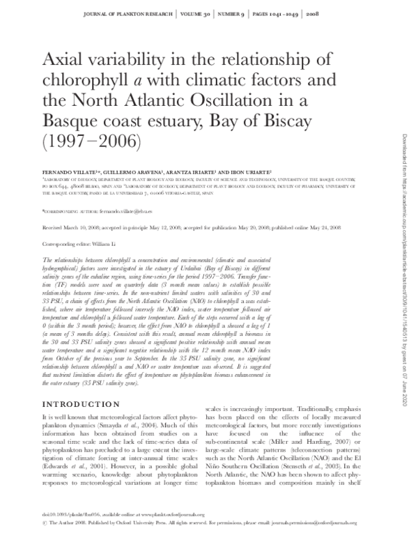METHOD Study area The estuary of Urdaibai (438220 N, 28430 W), also called the estuary of Mundaka, is located on the Basque coast, in the inner Bay of Biscay, within the middle latitudes of the eastern North Atlantic (Fig. 1). This area is influenced by the Gulf Stream and the atmospheric westerlies in the middle and upper troposphere; and the climate is temperate-oceanic with moderate winters and warm summers (Usabiaga et al., 2004). This estuary is a relatively short (12.5 km) and shallow (mean depth of 3 m) meso-macrotidal system. The central channel is bordered by salt marshes at its upper and middle reaches and by relatively extensive intertidal flats (mainly sandy) and sandy beaches at its lower reaches. The watershed area is relatively small in relation to the estuarine basin, and river inputs are usually low in relation to the tidal prism. In consequence, most of the estuary is marine-dominated, with high salinity waters in the outer half and a stronger axial gradient of salinity towards the head, where it receives most of the freshwater inputs from its main tributary, i.e. the Oka river. In the upper reaches, the estuary receives large amounts of nutrients and organic matter from a waste water treatment plant (Franco et al., 2004). In the outer zone, tidal flushing is high, to the 1042 Downloaded from https://academic.oup.com/plankt/article-abstract/30/9/1041/1540513 by guest on 07 June 2020 seas (Barton et al., 2003; Leterme et al., 2005). The nature of the relationship between NAO and phytoplankton, however, is claimed to vary within the North Atlantic, and this is partly due to the variety of environmental factors that the NAO can affect, e.g. temperature, water column stratification, currents and associated nutrients (Richardson and Schoeman, 2004; Leterme et al., 2005), and partly due to the geographic variability in the climatic expression (temperature and precipitation) of the NAO (Visbeck et al., 2001). Positive phases of the NAO index result in stronger westerly winds, increased precipitation and temperatures over northern Europe and south-eastern USA, but decreased precipitation and temperatures over northern Africa. Roughly, the opposite conditions correspond to negative phases of the NAO index (Visbeck et al., 2001). The Basque coast (northern Iberian peninsula) is located roughly at the border of these two climatically distinct regions, i.e. northern/central Europe and northern Africa. Previous studies have not shown a clear-cut picture of how the NAO relates to climate or to water temperature in the Basque coastal region (inner Bay of Biscay). While Saenz et al. (Saenz et al., 2001a) found no significant correlation between NAO and surface air temperature over the northern Iberian Peninsula, Garcı́a-Soto et al. (Garcı́a-Soto et al., 2002) showed winter sea surface temperature to be negatively correlated to NAO in the Cantabrian Sea (Bay of Biscay). Regarding possible effects of the NAO on phytoplankton, Beaugrand et al. (Beaugrand et al., 2000) showed no significant relationship between phytoplankton and the NAO in shelf edge and deep oceanic waters of the Bay of Biscay. However, the relationship has not been tested in estuarine waters. Being at the land – sea interface, many estuaries receive large amounts of nutrients that make them (or some zones within them) highly productive systems. The response of phytoplankton to temperature can be affected by nutrient availability (Rhee and Gotham, 1981; Geider et al., 1997). In many estuaries, strong spatial variations in nutrient concentrations can be found from the intermediate/inner to the outer zones and they can be ideal systems to test the hypothesis that phytoplankton response to climate is different in nutrient-replete and nutrient-limited waters. The estuary of Urdaibai, located on the Basque coast and draining into the Bay of Biscay, shows an axial gradient in nutrient concentrations, from the outer zone, which is nutrient-limited in summer, to the nutrient-rich intermediate and inner zones (Iriarte et al., 1996). In view of these considerations, we set out to investigate the following: (i) the relationship between the NAO index and the local climate on the Basque coast and its possible effect on water temperature; (ii) whether the 30 F. VILLATE ET AL. j AXIAL VARIABILITY IN THE RELATIONSHIP OF CHLOROPHYLL A Chlorophyll a values (mg L21) were transformed to log (x + 1) values to achieve homogeneity of variance. Air temperature, number of hours of sunshine, rainfall, NAO index and river flow data sets Statistical analyses Fig. 1. Map of the study area showing the location of the sampling zones. extent that waters of salinities .34 PSU are flushed out of the estuary with each tidal cycle (Villate et al., 1989). The outer half of the estuary remains well mixed most of the time, and the inner half is partially stratified. Chlorophyll a and water temperature data sets Monthly sampling was conducted from 1997 to 2006. Sampling was carried out during the last week of each month at high tide in the euhaline (salinity 30 PSU) region of the estuary. This estuarine region was chosen because river flow is relatively low in relation to the tidal prism and the euhaline waters constitute the main water body within the estuary at high tide (see Fig. 1 for location). Water samples were collected for chlorophyll a analysis from below the halocline (ca. mid depth) at three selected salinities: 30, 33 and 35 PSU. In the 30 PSU salinity zone, sampling commenced in 1999. At each sampling point, vertical profiles of temperature and salinity were obtained using WTW water quality meters. Chlorophyll a was measured spectrophotometrically according to the monochromatic method with acidification (Jeffrey and Mantoura, 1997). Occasional missing data in the time-series were interpolated using the Tramo-Seats package incorporated in the Demetra 2.0 interface, according to the methodology described by Gómez and Maravall (Gómez and Maravall, 1994) and Gómez et al. (Gómez et al., 1999). The method used for interpolation was the additive outlier (AO) approach with correction in the determinantal term of the likelihood (Gómez and Maravall, 1994). Given that the number of missing observations was not high (10%), this method gave similar results to the skipping approach, and the former was used following suggestions by Gómez and Maravall (Gómez and Maravall, 1994). To get a better picture of inter-annual variations, the seasonal component of air and water temperature, sunshine, rainfall, river flow and chlorophyll a series was removed by calculating the difference between the monthly value and the average for all years for each month divided by the standard deviation. This is a common procedure to deseasonalize time-series (e.g. Lehman, 2004). To better visualize inter-annual variations in the deseasonalized series, data were fitted using moving average curves (6 month period). To assess the relationships between NAO, climatic factors and chlorophyll a time-series, TF models were fitted using SAS 9.1 software, SAS Institute Inc. We used the TF methodology of Box and Jenkins (Box and Jenkins, 1976). Since, in most studies, seasonal NAO 1043 Downloaded from https://academic.oup.com/plankt/article-abstract/30/9/1041/1540513 by guest on 07 June 2020 Monthly mean air temperature, monthly accumulated rainfall and monthly number of cloudless hours were provided by the Spanish National Institute of Meteorology (Sondika) and the Provincial Council of Bizkaia (Muxika). The average values between data measured at the meteorological stations of Sondika and Muxika were taken. The number of hours of sunshine was only available from Sondika. Oka river flow data were provided by the Provincial Council of Bizkaia and correspond to the Muxika gauging station. Monthly NAO indices based on the difference in sea level pressure between Ponta Delgada, Azores (388N, 268W), and Akureyri, Iceland (668N, 188W), calculated by Rogers (Rogers, 1984) were taken from http:// polarmet.mps.ohio-state.edu/NAO/. JOURNAL OF PLANKTON RESEARCH j VOLUME indices are used, for the TF modelling quarterly mean (January–February–March, April–May–June, July– August–September and October–November–December) values were used for all variables, as has been done in other similar studies (e.g. Hänninen et al, 2003). The linear TF model can be written in the general form: uq ðBÞ vs ðBÞ ÞXtb þ ð Þat dr ðBÞ fp ðBÞ where Yt is the output series (the dependent variable); Xt the input series (the independent variable); C the constant term, vs(B) and dr(B) are the polynomial delay functions; B represents the backward shift operator and b is the delay time before Xt begins to influence Yt . The parameter fp is the autoregressive (AR) operator in non-seasonal series, and uq represents the moving average operator (MA). Here, at corresponds to the errors that are independently and identically distributed with normal distribution. In order to take care of non-stationary mean and variance, the response variable (output) and the explanatory variable (input) must, if necessary, be appropriately transformed. In the present work, where most series have a strong seasonal behaviour, a difference of order 4 (1 year) has been applied. According to the Box and Jenkins (1976) methodology, TF modelling is a three-step procedure. In the first step, the cross-correlation function (CCF) is used to identify the model. For the CCF to be meaningful, the input and output series must be filtered with a prewhitened model in order to reduce the residuals to white noise. The filter used for the output series must be the filter derived from the univariate analysis of the input variable. The use of prewhitened series to calculate the CCF is fundamental to reveal the existence of underlying relationships apart from the seasonal behaviour of the data. In the second step, the estimation of the model is carried out using the maximum likelihood methods and, finally, the diagnosis of the model is done using standard test statistics such as the modified Ljung-Box test (Stoffer and Toloi, 1992). For a more detailed description of the methodology, see Box and Jenkins (Box and Jenkins, 1976). The relationship between variables was also tested using parametric regression analysis. Linear regressions of chlorophyll a concentration on water temperature and NAO index were performed by the method of “least squares” using SPSS 15.0 software on normalized data. j NUMBER 9 j PAGES 1041 – 1049 j 2008 R E S U LT S Data showed a longitudinal gradient in chlorophyll a concentration in the euhaline region of the Urdaibai estuary (Figs 2–4), decreasing from the inner 30 PSU salinity zone (peak values ca. 25 mg L21) to the intermediate 33 PSU salinity zone (peak values ca. 12 mg L21) and to the outer 35 PSU salinity zone (peak values ca. 4 mg L21). The seasonal pattern of chlorophyll a concentration showed axial variations. In the 30 and 33 PSU salinity zones, it was a unimodal cycle with annual maxima in summer, whereas in the outer 35 salinity zone, chlorophyll a exhibited a bimodal cycle, with a spring maximum and a secondary peak in late summer–early autumn (Fig. 5). The inter-annual variations in the deseasonalized time-series (Figs. 2–4 and 6) showed great similarities for chlorophyll a at salinities of 30 and 33 PSU, water temperature at the three salinities tested and air temperature. The trend for the NAO index was roughly opposite (Fig. 6). The pattern of variation of other meteorological and hydrological variables studied (rainfall, number of cloudless hours and river flow) did not show a correspondence with those of chlorophyll a, temperature or NAO index (Fig. 6). In the series, two years can be highlighted for their meteorological features. In 2002, the NAO index was dominantly positive, whereas that of 2003 was mainly negative. Accordingly, 2002 was cooler than other years and 2003 was the warmest of the series. Chlorophyll a concentrations were lower than usual at salinities of 30 and 33 PSU during 2002 and were high in 2003. After this graphical analysis of the series, TF models were performed to test if there are statistically significant relationships between chlorophyll a concentration, environmental factors (air temperature, number of cloudless hours, rainfall, river flow and water temperature) and NAO index. Only results of the TF models Fig. 2. Time-series of chlorophyll a and water temperature in the 30 PSU salinity zone (left). Deseasonalized time-series of chlorophyll a and water temperature in the 30 PSU salinity zone (thin lines) and their corresponding moving averages (thick lines) (right). 1044 Downloaded from https://academic.oup.com/plankt/article-abstract/30/9/1041/1540513 by guest on 07 June 2020 Yt ¼ C þ ð 30 F. VILLATE ET AL. j AXIAL VARIABILITY IN THE RELATIONSHIP OF CHLOROPHYLL A Fig. 4. Time-series of chlorophyll a and water temperature in the 35 PSU salinity zone (left). Deseasonalized time-series of chlorophyll a and water temperature in the 35 PSU salinity zone (thin lines) and their corresponding moving averages (thick lines) (right). that showed significant (P , 0.05) correlations between time-series are shown in Table I, with the exception of the relationship between NAO index and chlorophyll a for the 30 PSU salinity zone, which was just below the significance level (P = 0.057). The corresponding CCFs have been plotted in Figs 7 and 8, in order to show the lag time of the response of one variable to another. From the TF modelling results, we can see that chlorophyll a concentration showed a positive response to water temperature at salinities of 30 PSU (t = 3.21, P = 0.003) and 33 PSU (t = 3.82, P , 0.001), but not at salinities of 35 PSU (Table I). In addition, a low quarterly NAO index was related with increased air temperature and this, in turn, was directly connected with water temperature at all the salinities tested (Table I). All these significant relationships showed a lag of 0 (i.e. effect within the same quarter) (Figs 7 and 8). This means that in the estuary of Urdaibai at salinities of 30 and 33 PSU, a chain of effects could be observed from NAO to air temperature to water Fig. 6. Time-series of monthly NAO index, surface air temperature, number of cloudless hours, rainfall and river flow (left). Deseasonalized time-series of surface air temperature, number of cloudless hours, rainfall and river flow (thin lines) and their corresponding moving averages (thick lines) (right). The NAO index series shows no seasonality and the thin line corresponds to the raw series. temperature and to chlorophyll a. TF modelling also revealed a negative relationship between chlorophyll a concentration and the NAO index (t = 24.06, P , 0.001) in waters of salinity of 33 PSU with a lag time of 1, i.e. chlorophyll a increases were detected in the following 1045 Downloaded from https://academic.oup.com/plankt/article-abstract/30/9/1041/1540513 by guest on 07 June 2020 Fig. 3. Time-series of chlorophyll a and water temperature in the 33 PSU salinity zone (left). Deseasonalized time-series of chlorophyll a and water temperature in the 33 PSU salinity zone (thin lines) and their corresponding moving averages (thick lines) (right). Fig. 5. Seasonal pattern of chlorophyll a in the 30 (dashed), 33 (solid) and 35 (dotted) PSU salinity waters. To calculate the deviations, the annual median was removed from each monthly value, leaving a time-series of deviations for each month from the annual median for that year. The median seasonal pattern was found by using the median of each monthly deviation for all years. JOURNAL OF PLANKTON RESEARCH j VOLUME 30 j NUMBER 9 j PAGES 1041 – 1049 j 2008 Table I: Transfer function model results, showing the relationships between time-series Variable Lag b t P-value NAO versus air temperature NAO 0 20.795 24.82 ,0.001 Air temperature versus water temperature salinity 30 AR1,1 Air temp 4 0 20.699 24.60 ,0.001 0.279 2.18 0.039 Air temperature versus water temperature, salinity 33 MA1,1 Air temp 4 0 Air temperature versus water temperature, salinity 35 AR1,1 Air temp 4 0 Water temperature versus chlorophyll a, salinity 30 MA1,1 4 Wat temp 0 Water temperature versus chlorophyll a, salinity 33 AR1,1 4 Wat temp 0 0.581 0.370 4.01 ,0.001 3.35 0.002 0.834 0.113 5.99 ,0.001 3.21 0.004 20.690 24.76 ,0.001 0.102 3.82 0.001 NAO versus chlorophyll a, salinity 30 MA1,1 NAO 4 1 0.757 4.83 ,0.001 20.078 22.01 0.057 NAO versus chlorophyll a, salinity 33 NAO 1 20.089 24.06 0.001 All the time-series contain quarterly mean values for the period 1997 – 2005, except those of water temperature and chlorophyll a at 30 PSU salinity, which extend from 1999 to 2005 (b is the parameter estimate, t the statistic, MA1,1 the moving average term and AR1,1 the AR term). quarter (Table I and Fig. 8). Chlorophyll a and NAO index in waters of salinity of 30 PSU were only weakly correlated according to the CCFs (Fig. 8), and the TF model regression was nearly significant (Table I). Regression analyses (Fig. 9) showed annual mean chlorophyll a concentration to be positively and significantly related to annual mean water temperature at salinities of 30 PSU (P = 0.013) and 33 PSU (P = 0.003) and to be negatively and significantly related to the NAO index averaged from October of the previous year to September also at salinities of 30 PSU (P = 0.048) and 33 PSU (P , 0.001). The NAO index that we used reflects the lagged effect of the NAO on chlorophyll a shown by the TF models. DISCUSSION The NAO is claimed to have a roughly opposite climate expression (surface air temperature and precipitation) in northern/central Europe and northern Africa (Visbeck et al., 2001). The Basque coast seems to be located in a transition zone between the two. Previous studies conducted in the area have shown contradictory results. Saenz et al. (Saenz et al., 2001a) reported no correlation between a winter NAO index and surface air temperature in the northern Iberian Peninsula, but this study was conducted over a broader geographical area, and Fig. 7. CCF to lag 5 for the prewhitened time-series (air temperature versus NAO index, water temperature versus air temperature at the 30, 33 and 35 PSU salinity waters). Standard error limits are shown as broken lines. The TF analysis was performed grouping data in quarterly means (see text for further details). temperature variations from inland to coastal sites within the northern Iberian Peninsula can be significant, due, among others, to Föehn effects (Saenz et al., 2001a). In contrast, Garcı́a-Soto et al. (Garcı́a-Soto et al., 2002) showed winter water warming during marked Navidad years to be negatively correlated with a November– December NAO index. Our TF modelling results have shown that on the Basque coast, in relation to temperature, the NAO has a Mediterranean-like expression, where positive phases of the NAO result in decreased surface air temperatures and these, in turn, result in decreased water temperatures. The NAO index, however, showed no significant correlation with precipitation, which is in accordance with results from other studies for the north-eastern area of the Iberian 1046 Downloaded from https://academic.oup.com/plankt/article-abstract/30/9/1041/1540513 by guest on 07 June 2020 20.576 23.56 0.001 0.333 3.70 ,0.001 F. VILLATE ET AL. j AXIAL VARIABILITY IN THE RELATIONSHIP OF CHLOROPHYLL A Fig. 9. Relationship between annual mean chlorophyll a concentration and annual mean water temperature (top). Relationship between annual mean chlorophyll a concentration and NAO index averaged from October of the previous year to September (bottom). Grey, dark and open circles represent the 30, 33 and 35 PSU salinity waters, respectively. Peninsula, including both the Cantabrian and the Mediterranean coasts (Rodó et al., 1997; Saenz et al., 2001b). The time-series analysed in our study only covers a decade; however, these results hold when tested for a longer (30 year) period (Aravena et al., unpublished data). According to the TF results from the present work, the NAO effect on water temperature was strong enough to affect phytoplankton biomass at salinities of 30 and 33 PSU and this was best shown as a chain of effects from NAO to air temperature, to water temperature and to chlorophyll a, although it was also evident when we tested the relationship between the time-series of the NAO and chlorophyll a in the 33 PSU waters, the latter showing a lag that was not apparent in the sequential relationships within the chain. The almost significant TF 1047 Downloaded from https://academic.oup.com/plankt/article-abstract/30/9/1041/1540513 by guest on 07 June 2020 Fig. 8. As in Fig. 6 for chlorophyll a versus water temperature and chlorophyll a versus NAO index in the 30 and 33 PSU salinity waters. model (P = 0.057) of NAO versus chlorophyll a obtained for waters of 30 PSU of salinity was likely due to the smaller number of data points available for this salinity zone. Consistent with the TF results, regression analysis showed that annual mean chlorophyll a concentration at salinities of 30 and 33 PSU was positively correlated with annual mean water temperature and negatively with the NAO index averaged from October of the previous year to September. Significant relationships between the NAO and phytoplankton biomass have been reported in different areas across the North Atlantic, particularly in shelf waters (Barton et al., 2003; Leterme et al., 2005). However, the relationship between the NAO and phytoplankton biomass is not always negative as in some zones within the estuary of Urdaibai, and appears to be site-specific. The complexity of the NAO – phytoplankton relationship is often explained in terms of the variety of indirect impacts that the NAO can have on the physico-chemical characteristics of seawater, via temperature, water column mixing and currents, and associated changes in nutrients (Leterme et al., 2005). For example, Richardson and Schoeman (2004) found that in the Northeast Atlantic, in turbulent, nutrient-rich, cool waters, warming can enhance phytoplankton biomass by increasing metabolic rates and stratification, whereas in stratified-nutrient-poor warm waters warming can cause phytoplankton biomass to decrease because it enhances existing stratification and limits access to nutrients. In agreement with this finding, Edwards et al. (Edwards et al., 2001) found that NAO shows a positive correlation with dinoflagellates, but negative with diatoms. The complexity of the relationship between the NAO and chlorophyll a can also be seen in estuaries and bays. Thus, Belgrano et al. (Belgrano et al., 1999) found a positive correlation between winter NAO and spring phytoplankton biomass/primary production in the Gullmar Fjord (Sweden), which they explained in terms of variations in water circulation caused by the NAO. For Narragansett Bay, however, Smayda et al. (Smayda et al., 2004) reported a negative relationship between annual mean NAO and annual mean chlorophyll a concentration, which they attributed to temperature-dependent changes in grazing. Also, in Narragansett Bay, in addition to effects caused by temperature changes, the NAO effect is also likely related to modifications in hydrography. In the estuary of Urdaibai, water circulation and mixing is governed by tides and river discharge. Therefore, it is unlikely that the increase in phytoplankton biomass following increases in temperature is related to modifications of currents caused by NAO. We hypothesize that direct temperature effects causing JOURNAL OF PLANKTON RESEARCH j VOLUME j NUMBER 9 j PAGES 1041 – 1049 j 2008 warmest period of the year (Ruiz et al., 1998). Temperature and nutrient availability have a combined effect on phytoplankton growth (Rhee and Gotham, 1981; Geider et al., 1997). We suggest that in the outer estuary of Urdaibai, nutrient limitation prevents phytoplankton biomass responding to temperature variations in the way it does in nutrient-rich zones of the estuary. Iron limitation has been suggested to interact with the temperature dependence of phytoplankton growth in the Pacific ocean (Nori et al., 2005) and resource limitation has also been shown to distort the temperature dependence of bacterial metabolism in the oceans (López-Urrutia and Morán, 2007). In agreement with our findings for the 35 PSU salinity waters of the estuary of Urdaibai, a study conducted in shelf edge and deep oceanic waters of the Bay of Biscay showed no significant relationship between phytoplankton and the NAO (Beaugrand et al., 2000). We believe that in the Urdaibai estuary, the NAO only induces significant variations in chlorophyll a concentration in non-nutrient limited waters, such as the intermediate and inner zones of the estuary, where chlorophyll a peaks occur in the warmest season. Results from the present study can contribute to fill a geographic gap in the knowledge of the NAO effects on phytoplankton in the North Atlantic, and warn of the enhancement of eutrophication that could occur with global warming in nonnutrient limited estuarine waters. AC K N OW L E D G E M E N T S We would like to thank Dr. Berta Ibañez for assistance with the transfer function modelling. Thanks are also due to the Provincial Council of Bizkaia for providing meteorological and river flow data. FUNDING Financial support for this research was provided predominantly by the UNESCO Chair on “Sustainable Development and Environmental Education” (UNESCO 03/04), the University of the Basque Country (EHU06/ 52) and by the Department of Industry, Commerce and Tourism of the Basque Government (ETORTEK07/25). G.A. acknowledges the receipt of a PhD grant from the University of the Basque Country. REFERENCES Barton, A. D., Greene, C. H., Monger, B. C. et al. (2003) The Continuous Plankton Recorder survey and the North Atlantic Oscillation: interannual- to multidecadal-scale patterns of phytoplankton variability in the North Atlantic Ocean. Prog. Oceanogr., 58, 337–358. 1048 Downloaded from https://academic.oup.com/plankt/article-abstract/30/9/1041/1540513 by guest on 07 June 2020 increases in metabolic rates and indirect ones enhancing existing water column stratification, and hence improving phytoplankton cell light quota, are the main mechanisms involved. The fact that the climatic expression of NAO varies geographically within the North Atlantic (Hurrell and van Loom, 1997) adds a further source of variability to the NAO versus chlorophyll a relationship. Over the Basque coast, positive phases of the NAO are linked to decreases in air temperature, so even if in the 30 – 33 PSU salinity zone of the estuary of Urdaibai, phytoplankton biomass is positively linked to temperature, as is the case, for example, in areas at higher latitudes in Central North Atlantic (Barton et al., 2003), the relationship between NAO and phytoplankton show opposite signs, negative in the estuary of Urdaibai and positive in Central North Atlantic. A given change in the NAO seems to result in similar changes in chlorophyll a in the estuary of Urdaibai and in estuaries in other areas in the North Atlantic. For example, making a rough calculation with data taken from Figure 4.3 in Smayda et al. (2004), in Narragansett Bay, a decrease of 2 units in the annual NAO index results in a 2.5-fold increase in chlorophyll a, and in the estuary of Urdaibai a decrease of 2 units in the mean October– September NAO index would also result in a 2.5-fold increase in the annual mean chlorophyll a (averaged for the 30 and 33 salinity zones). In addition, results from the present work show that in estuaries we can also find axial variations in the relationship between chlorophyll a concentration and NAO/water temperature. Significant links between water temperature and chlorophyll a concentration were detected at salinities of 30 and 33 PSU, but not at salinities of 35 PSU. Water masses of salinities between 30 and 33 PSU located below the halocline remain within the estuary at low tide, whereas those of 35 PSU are flushed out of the estuary with each tidal cycle (Villate et al., 1989). As a consequence, in summer, nutrients become limiting (sensu Fisher et al., 1988) for phytoplankton growth in the outer estuary whereas the intermediate and inner zones are not nutrient-limited (Iriarte et al., 1996). The nutrient limitation at the 35 salinity zone in summer is corroborated by the bimodal seasonal pattern of chlorophyll a concentration, with a summer decrease between the spring and late summer– early autumn peaks, in contrast with the summer annual-maxima found in the 30 and 33 salinity zones. A previous study carried out with a high-frequency sampling programme (every 3 days) during July and August showed that the marked decrease of phytoplankton biomass from the 33 to the 35 salinity waters of the estuary of Urdaibai is a consistent pattern during the 30 F. VILLATE ET AL. j AXIAL VARIABILITY IN THE RELATIONSHIP OF CHLOROPHYLL A Beaugrand, G., Ibañez, F. and Reid, P. C. (2000) Spatial, seasonal, and long-term fluctuations of plankton in relation to hydroclimatic features in the English Channel, Celtic Sea and Bay of Biscay. Mar. Ecol. Prog. Ser., 200, 93– 102. Belgrano, A., Lindhal, O. and Hernroth, B. (1999) North Atlantic Oscillation, primary productivity and toxic phytoplankton in the Gullmar Fjord, Sweden (1985–1996). Proc. R. Soc. Lond. B, 266, 425–430. Bhangu, I. and Whitfield, P. H. (1997) Seasonal and long-term variation in water quality of the Skeena river at Usk, British Columbia. Wat. Res., 31, 2187– 2194. Edwards, M., Reid, P. C. and Planque, B. (2001) Long-term and regional variability of phytoplankton biomass in the north-east Atlantic (1960– 1995). ICES J. Mar. Sci., 58, 39– 49. Fisher, T. R., Harding, L. W., Jr., Stanley, D. W. et al. (1988) Phytoplankton, nutrients and turbidity in the Chesapeake, Delaware and Hudson Estuaries. Estuar. Coast. Shelf Sci., 27, 61– 93. Franco, J., Borja, A. and Valencia, V. (2004) Overall assessment—human impacts and quality status. In Borja, A. and Collins, M. (eds), Oceanography and Marine Environment of the Basque Country. Elsevier Oceanography Series 70, Elsevier, Amsterdam, pp. 581–597. Garcı́a-Soto, C., Pingree, R. D. and Valdés, L. (2002) Navidad development in the southern Bay of Biscay: climate change and swoody structure from remote sensing and in situ measurements. J. Geophys. Res., 107, doi:101029/2001JC001012 Geider, R. J., MacIntyre, H. L. and Kana, T. M. (1997) Dynamic model of phytoplankton growth and acclimation: responses of the balanced growth rate and the chlorophyll a:carbon ratio to light, nutrient-limitation and temperature. Mar. Ecol. Prog. Ser., 148, 187–200. Gómez, V. and Maravall, A. (1994) Estimation, prediction, and interpolation for nonstationary series with the Kalman filter. J. Am. Stat. Assoc., 89, 611– 624. Gómez, V., Maravall, A. and Peña, D. (1999) Missing observations in ARIMA models: skipping approach versus additive outlier approach. J. Econometrics, 88, 341–363. Hänninen, J., Vuorinen, I. and Kornilovs, G. (2003) Atlantic climatic factors control decadal dynamics of a Baltic Sea copepod Temora longicornis. Ecography, 26, 672–678. Hurrel, J. W. and van Loom, H. (1997) Decadal variations in climate associated with the North Atlantic Oscillation. Clim. Change, 36, 301–326. Iriarte, A., Madariaga, I. de, Diez-Garagarza, F. et al. (1996) Primary plankton production, respiration and nitrification in a shallow temperate estuary during summer. J. Exp. Mar. Biol. Ecol., 208, 127–151. Jeffrey, S. W. and Mantoura, R. F. C. (1997) Development of pigment methods for oceanography: SCOR-supported Working Groups and objectives. In Jeffrey, S. W., Mantoura, R. F. C. and Wright, S. W. (eds), Phytoplankton Pigments in Oceanography: Guidelines to Modern Methods. UNESCO, Paris, pp. 19–36. López-Urrutia, A. and Morán, X. A. G. (2007) Resource limitation of bacterial production distorts the temperature dependence of oceanic carbon cycling. Ecology, 88, 817–822. Miller, W. D. and Harding, L. W., Jr. (2007) Climate forcing of the spring bloom in Chesapeake Bay. Mar. Ecol. Prog. Ser., 331, 11–22. Nori, Y., Kudo, I., Kiyosawa, H. et al. (2005) Influence of iron and temperature on growth, nutrient utilization ratios and phytoplankton species composition in the western subarctic Pacific Ocean during the SEEDS experiment. Prog. Oceanogr., 64, 149 –166. Rhee, G.-Y. and Gotham, I. J. (1981) The effect of environmental factors on phytoplankton growth: temperature and the interactions of temperature with nutrient limitation. Limnol. Oceanogr., 26, 635–648. Richardson, A. J. and Schoeman, D. S. (2004) Climate impact on plankton ecosystems in the Northeast Atlantic. Science, 305, 1609–1612. Rodó, X., Baert, E. and Comı́n, F. A. (1997) Variations in seasonal rainfall in Southern Europe during the present century: relationships with The North Atlantic Oscillation and the El Niño-Southern Oscillation. Clim. Dyn., 13, 275– 284. Rogers, J. C. (1984) The association between the North Atlantic Oscillation and the Southern Oscillation in the northern hemisphere. Mon. Weather Rev., 112, 1999– 2015. Ruiz, A., Franco, J. and Villate, F. (1998) Microzooplankton grazing in the Estuary of Mundaka, Spain, and its impact on the phytoplankton distribution along the salinity gradient. Aquat. Microb. Ecol., 14, 281–288. Saenz, J., Zubillaga, J. and Rodrı́guez-Puebla, C. (2001a) Interannual winter temperature variability in the north of the Iberian Peninsula. Clim. Res., 16, 169 –179. Saenz, J., Zubillaga, J. and Rodrı́guez-Puebla, C. (2001b) Interannual variability of winter precipitation in northern Iberian Peninsula. Int. J. Climatol, 21, 1503– 1513. Smayda, T. J., Borkman, D. G., Beaugrand, G. et al. (2004) Responses of marine phytoplankton populations to fluctuations in marine climate. In Stenseth, N. C., Ottersen, G., Hurrell, J. W., Belgrano, A. et al. (eds), Marine Ecosystems and Climate Variation. Oxford University Press, Oxford, pp. 49–58. Stenseth, N. C., Ottersen, G., Hurrell, J. W. et al. (2003) Studying climate effects on ecology through the use of climate indices: the North Atlantic Oscillation, El Niño Southern Oscillation and beyond. Proc. R. Soc. Lond. B, 270, 2087–2096. Stoffer, D. and Toloi, C. (1992) A note on the Ljung-Box-Pierce Portmanteau statistics with missing data. Stat. Probab. Lett., 13, 391–396. Usabiaga, J. I., Saenz Aguirre, J., Valencia, V. et al. (2004) Climate and meteorology, variability and its influence on the ocean. In Borja, A. and Collins, M. (eds), Oceanography and Marine Environment of the Basque Country. Elsevier Oceanography Series 70, Elsevier, Amsterdam, pp. 75–95. Villate, F., Franco, J., Ruiz, A. et al. (1989) Caracterización geomorfológica e hidrológica de cinco sistemas estuáricos del Paı́s Vasco. Kobie, 18, 157–170. Lehman, P. W. (2004) The influence of climate on mechanistic pathways that affect lower food web production in northern San Francisco Bay estuary. Estuaries, 27, 311– 324. Visbeck, M. H., Hurrell, J. W., Polvani, L. et al. (2001) The North Atlantic Oscillation: past, present and future. Proc. Natl Acad. Sci. USA, 98, 12876– 12877. Lehmann, A. and Rode, M. (2001) Long-term behaviour and crosscorrelation water quality analysis of the river Elbe, Germany. Wat. Res., 35, 2153– 2160. Vuorinen, I., Hänninen, J. and Kornilovs, G. (2003) Transfer-function modelling between environmental variation and mesozooplankton in the Baltic Sea. Prog. Oceanogr., 59, 339–356. 1049 Downloaded from https://academic.oup.com/plankt/article-abstract/30/9/1041/1540513 by guest on 07 June 2020 Box, G. E. P. and Jenkins, G. M. (1976) Time Series Analysis: Forecasting and Control. Holden-Day, San Francisco. Leterme, S. C., Edwards, M., Seuront, L. et al. (2005) Decadal basinscale changes in diatoms, dinoflagellates, and phytoplankton color across the North Atlantic. Limnol. Oceanogr., 50, 1244– 1253.