Q-learning is a model-free reinforcement learning algorithm that helps an agent learn the optimal action-selection policy by iteratively updating Q-values, which represent the expected rewards of actions in specific states.
The article aims to explain Q-learning, a key reinforcement learning algorithm, by detailing its components, working principles, and applications across various fields.
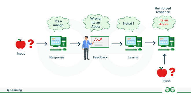
Reinforcement Learning is a paradigm of the Learning Process in which a learning agent learns, over time, to behave optimally in a certain environment by interacting continuously in the environment. The agent during its course of learning experiences various situations in the environment it is in. These are called states. The agent while being in that state may choose from a set of allowable actions which may fetch different rewards (or penalties). Over time, The learning agent learns to maximize these rewards to behave optimally at any given state it is in. Q-learning is a basic form of Reinforcement Learning that uses Q-values (also called action values) to iteratively improve the behavior of the learning agent.
This example helps us to better understand reinforcement learning.
Q-Learning
Q-learning in Reinforcement Learning
Q-learning is a popular model-free reinforcement learning algorithm used in machine learning and artificial intelligence applications. It falls under the category of temporal difference learning techniques, in which an agent picks up new information by observing results, interacting with the environment, and getting feedback in the form of rewards.
Key Components of Q-learning
1. Q-Values or Action-Values
Q-values are defined for states and actions. [Tex]Q(S, A)
[/Tex] is an estimation of how good is it to take the action A at the state S . This estimation of [Tex]Q(S, A)
[/Tex] will be iteratively computed using the TD- Update rule which we will see in the upcoming sections.
2. Rewards and Episodes
An agent throughout its lifetime starts from a start state, and makes several transitions from its current state to a next state based on its choice of action and also the environment the agent is interacting in. At every step of transition, the agent from a state takes an action, observes a reward from the environment, and then transits to another state. If at any point in time, the agent ends up in one of the terminating states that means there are no further transitions possible. This is said to be the completion of an episode.
3. Temporal Difference or TD-Update
The Temporal Difference or TD-Update rule can be represented as follows:
[Tex]Q(S,A)\leftarrow Q(S,A) + \alpha (R + \gamma Q({S}’,{A}’) – Q(S,A))
[/Tex]
This update rule to estimate the value of Q is applied at every time step of the agent’s interaction with the environment. The terms used are explained below:
- S: Current State of the agent.
- A: Current Action Picked according to some policy.
- S’: Next State where the agent ends up.
- A’: Next best action to be picked using current Q-value estimation, i.e. pick the action with the maximum Q-value in the next state.
- R: Current Reward observed from the environment in Response of current action.
- [Tex]\gamma
[/Tex](>0 and <=1) : Discounting Factor for Future Rewards. Future rewards are less valuable than current rewards so they must be discounted. Since Q-value is an estimation of expected rewards from a state, discounting rule applies here as well.
- [Tex]\alpha
[/Tex]: Step length taken to update the estimation of Q(S, A).
4. Selecting the Course of Action with ϵ-greedy policy
A simple method for selecting an action to take based on the current estimates of the Q-value is the ϵ-greedy policy. This is how it operates:
Superior Q-Value Action (Exploitation):
- With a probability of 1−ϵ, representing the majority of cases,
- Select the action with the highest Q-value at the moment.
- In this instance of exploitation, the agent chooses the course of action that, given its current understanding, it feels is optimal.
Exploration through Random Action:
- With probability ϵ, occasionally,
- Rather than selecting the course of action with the highest Q-value,
- Select any action at random, irrespective of Q-values.
- In order to learn about the possible benefits of new actions, the agent engages in a type of exploration.
How does Q-Learning Works?
Q-learning models engage in an iterative process where various components collaborate to train the model. This iterative procedure encompasses the agent exploring the environment and continuously updating the model based on this exploration.
The key components of Q-learning include:
- Agents: Entities that operate within an environment, making decisions and taking actions.
- States: Variables that identify an agent’s current position in the environment.
- Actions: Operations undertaken by the agent in specific states.
- Rewards: Positive or negative responses provided to the agent based on its actions.
- Episodes: Instances where an agent concludes its actions, marking the end of an episode.
- Q-values: Metrics used to evaluate actions at specific states.
Methods for Determining Q-Values
There are two methods for determining Q-values:
- Temporal Difference: Calculated by comparing the current state and action values with the previous ones.
- Bellman’s Equation: A recursive formula invented by Richard Bellman in 1957, used to calculate the value of a given state and determine its optimal position. It provides a recursive formula for calculating the value of a given state in a Markov Decision Process (MDP) and is particularly influential in the context of Q-learning and optimal decision-making.
Bellman’s Equation is expressed as :
[Tex]Q(s,a) = R(s,a) + \gamma \;\; max_a Q(s’,a)[/Tex]
Where,
- Q(s,a) is the Q-value for a given state-action pair
- R(s,a) is the immediate reward for taking action a in state s.
- gamma is the discount factor, representing the importance of future rewards.
- maxaQ(s′,a) is the maximum Q-value for the next state ′s′ and all possible actions.
What is Q-table?
The Q-table is a repository of rewards associated with optimal actions for each state in a given environment. It serves as a guide for the agent, helping it determine which actions are likely to yield the best outcomes. As the agent interacts with the environment, the Q-table is dynamically updated to reflect the agent’s evolving understanding, enabling more informed decision-making.
Implementation of Q-Learning
Step 1: Define the Environment
Set up the environment parameters, including the number of states and actions, and initialize the Q-table. In this grid world, each state represents a position, and actions move the agent within this environment.
import numpy as np
# Define the environment
n_states = 16 # Number of states in the grid world
n_actions = 4 # Number of possible actions (up, down, left, right)
goal_state = 15 # Goal state
# Initialize Q-table with zeros
Q_table = np.zeros((n_states, n_actions))
Step 2: Set Hyperparameters
Define the parameters for the Q-learning algorithm, including the learning rate, discount factor, exploration probability, and the number of training epochs.
# Define parameters
learning_rate = 0.8
discount_factor = 0.95
exploration_prob = 0.2
epochs = 1000
Step 3: Implement the Q-Learning Algorithm
Perform the Q-learning algorithm over multiple epochs. Each epoch involves selecting actions based on an epsilon-greedy strategy, updating Q-values based on rewards received, and transitioning to the next state.
# Q-learning algorithm
for epoch in range(epochs):
current_state = np.random.randint(0, n_states) # Start from a random state
while current_state != goal_state:
# Choose action with epsilon-greedy strategy
if np.random.rand() < exploration_prob:
action = np.random.randint(0, n_actions) # Explore
else:
action = np.argmax(Q_table[current_state]) # Exploit
# Simulate the environment (move to the next state)
# For simplicity, move to the next state
next_state = (current_state + 1) % n_states
# Define a simple reward function (1 if the goal state is reached, 0 otherwise)
reward = 1 if next_state == goal_state else 0
# Update Q-value using the Q-learning update rule
Q_table[current_state, action] += learning_rate * \
(reward + discount_factor *
np.max(Q_table[next_state]) - Q_table[current_state, action])
current_state = next_state # Move to the next state
Step 4: Output the Learned Q-Table
After training, print the Q-table to examine the learned Q-values, which represent the expected rewards for taking specific actions in each state.
# After training, the Q-table represents the learned Q-values
print("Learned Q-table:")
print(Q_table)
Implement Q-Algorithm
Python
import numpy as np

# Define the environment
n_states = 16  # Number of states in the grid world
n_actions = 4  # Number of possible actions (up, down, left, right)
goal_state = 15  # Goal state

# Initialize Q-table with zeros
Q_table = np.zeros((n_states, n_actions))

# Define parameters
learning_rate = 0.8
discount_factor = 0.95
exploration_prob = 0.2
epochs = 1000

# Q-learning algorithm
for epoch in range(epochs):
    current_state = np.random.randint(0, n_states)  # Start from a random state

    while current_state != goal_state:
        # Choose action with epsilon-greedy strategy
        if np.random.rand() < exploration_prob:
            action = np.random.randint(0, n_actions)  # Explore
        else:
            action = np.argmax(Q_table[current_state])  # Exploit

        # Simulate the environment (move to the next state)
        # For simplicity, move to the next state
        next_state = (current_state + 1) % n_states

        # Define a simple reward function (1 if the goal state is reached, 0 otherwise)
        reward = 1 if next_state == goal_state else 0

        # Update Q-value using the Q-learning update rule
        Q_table[current_state, action] += learning_rate * \
            (reward + discount_factor *
             np.max(Q_table[next_state]) - Q_table[current_state, action])

        current_state = next_state  # Move to the next state

# After training, the Q-table represents the learned Q-values
print("Learned Q-table:")
print(Q_table)
Output:
Learned Q-table:
[[0.48767498 0.48377358 0.48751874 0.48377357]
[0.51252074 0.51317781 0.51334071 0.51334208]
[0.54036009 0.5403255 0.54018713 0.54036009]
[0.56880009 0.56880009 0.56880008 0.56880009]
[0.59873694 0.59873694 0.59873694 0.59873694]
[0.63024941 0.63024941 0.63024941 0.63024941]
[0.66342043 0.66342043 0.66342043 0.66342043]
[0.6983373 0.6983373 0.6983373 0.6983373 ]
[0.73509189 0.73509189 0.73509189 0.73509189]
[0.77378094 0.77378094 0.77378094 0.77378094]
[0.81450625 0.81450625 0.81450625 0.81450625]
[0.857375 0.857375 0.857375 0.857375 ]
[0.9025 0.9025 0.9025 0.9025 ]
[0.95 0.95 0.95 0.95 ]
[1. 1. 1. 1. ]
[0. 0. 0. 0. ]]
The Q-learning algorithm involves iterative training where the agent explores and updates its Q-table. It starts from a random state, selects actions via epsilon-greedy strategy, and simulates movements. A reward function grants a 1 for reaching the goal state. Q-values update using the Q-learning rule, combining received and expected rewards. This process continues until the agent learns optimal strategies. The final Q-table represents acquired state-action values after training.
Advantages of Q-learning
- Long-term outcomes, which are exceedingly challenging to accomplish, are best achieved with this strategy.
- This learning paradigm closely resembles how people learn. Consequently, it is almost ideal.
- The model has the ability to fix mistakes made during training.
- Once a model has fixed a mistake, there is virtually little probability that it will happen again.
- It can produce the ideal model to address a certain issue.
Disadvantages of Q-Learning
- Drawback of using actual samples. Think about the situation of robot learning, for instance. The hardware for robots is typically quite expensive, subject to deterioration, and in need of meticulous upkeep. The expense of fixing a robot system is high.
- Instead of abandoning reinforcement learning altogether, we can combine it with other techniques to alleviate many of its difficulties. Deep learning and reinforcement learning are one common combo.
Applications of Q-learning
Applications for Q-learning, a reinforcement learning algorithm, can be found in many different fields. Here are a few noteworthy instances:
- Atari Games: Classic Atari 2600 games can now be played with Q-learning. In games like Space Invaders and Breakout, Deep Q Networks (DQN), an extension of Q-learning that makes use of deep neural networks, has demonstrated superhuman performance.
- Robot Control: Q-learning is used in robotics to perform tasks like navigation and robot control. With Q-learning algorithms, robots can learn to navigate through environments, avoid obstacles, and maximise their movements.
- Traffic Management: Autonomous vehicle traffic management systems use Q-learning. It lessens congestion and enhances traffic flow overall by optimising route planning and traffic signal timings.
- Algorithmic Trading: The use of Q-learning to make trading decisions has been investigated in algorithmic trading. It makes it possible for automated agents to pick up the best strategies from past market data and adjust to shifting market conditions.
- Personalized Treatment Plans: To make treatment plans more unique, Q-learning is used in the medical field. Through the use of patient data, agents are able to recommend personalized interventions that account for individual responses to various treatments.
Frequently Asked Questions (FAQs) on Q-Learning
What is the Q-learning method?
Q-learning is a reinforcement learning algorithm that learns the optimal action-selection policy for an agent by updating Q-values, which represent the expected rewards of actions in given states.
What is the difference between R learning and Q-learning?
Q-learning focuses on maximizing the total expected reward, while R-learning is designed to maximize the average reward per time step, often used in continuing tasks.
Is Q-learning a neural network?
No, Q-learning itself is not a neural network, but it can be combined with neural networks in approaches like Deep Q-Networks (DQN) to handle complex, high-dimensional state spaces.