Section on Survey Research Methods – JSM 2008 Robust Estimation of Monthly Employment Growth Rates for Small Areas in the Current Employment Statistics Survey * 1 Julie Gershunskaya1 and Partha Lahiri2 U.S. Bureau of Labor Statistics, 2 Massachusetts Ave NE, Suite 4985, Washington, DC, 20212 2 University of Maryland, College Park Abstract Each month, the Bureau of Labor Statistics publishes estimates of employment for industrial supersectors at the metropolitan statistical area (MSA) level. The survey-weighted ratio estimator that is used to produce estimates for large domains is generally less reliable for MSA level estimation due to the unavailability of adequate sample from a given MSA. We also note that the effect of a few establishments, which are influential in terms of unusual employment numbers or sampling weights or both, could be prominent for the small area estimation. In this paper, we develop an empirical hierarchical Bayes method based on a unit level model. Our proposed method is found to be less variable and less sensitive to influential establishments when compared to the direct survey-weighted ratio estimator or estimators based on an area level model. Empirical evaluation of the estimators is performed using the population data from administrative file. Key Words: small area estimation, robust estimation, influential observations 1. Introduction Complex surveys are usually designed to collect enough sample units from a population of interest and to make estimates of population quantities based on this sample with a satisfactory precision. However, at a progressively finer level of detail, where the sample is sparse, direct sample based estimates could be highly imprecise. The problem of estimation at such detailed levels is known as small area estimation (SAE) problem. A model is formulated to “borrow strength” from additional sources (e.g., from the neighboring areas or historical data), to improve on the quality of the estimates for small areas. A thorough account of existing SAE methods is given in Rao (2003). In this paper, we consider the situation when the population parameter of interest is given in a pre-specified form; the motivation for the form of the target does not necessarily come from a stochastic model. For example, in application considered in this paper, we are interested in estimation of the ratio of two population means: levels of employment in the current and previous months. A somewhat more complex set of examples give various forms of the price indexes, important economic indicators published from surveys conducted by national governments. The definition of the price indexes can be motivated using a range of requirements that do not assume any stochastic nature of the population measurements. To estimate such pre-defined targets using a small sample, one may first derive estimates based on the sample and then stabilize them by applying an area-level SAE method, e.g., the Fay-Herriot model (Fay and Herriot 1979). In models of this type, assumptions are made on the area-level direct sample based estimates. In many situations, however, it is preferable to formulate model at a unit level. If the unit-level auxiliary information is available, a model that incorporates such information can be especially beneficial. However, there are reasons to consider a unit-level model even in the absence of such auxiliary data. In our application, we observe that the direct sample-based estimates can be heavily affected by the influential observations, which are common in the establishment surveys (see Hidiroglou 1994; Lee 1995; Rivest 1999; Section 3 of this paper). One problem with the area-level model is that the sampling variance of the direct sample based estimate, considered to be known, does not always properly reflect the existence of influential observations in a particular realized sample. If this is the case, the adverse effect from such units carries over onto the resulting model estimate. On the other hand, the * Any opinions expressed in this paper are those of the authors and do not constitute policy of the Bureau of Labor Statistics. 297 Section on Survey Research Methods – JSM 2008 effect from influential observations can be harnessed by fine-tuning the modeling assumptions on measurements at the unit level. When the form of the finite population target is pre-specified, a unit level model is naturally obtained by considering the effect of measurements from individual units on the estimator of the given form. In infinite population settings, Hampel (1974) introduced the notion of the influence function. The influence function measures the effect of small changes in the underlying distribution on the estimator. In other words, the approach allows assessment of the effect of individual observations on the estimated target quantity by linearizing the target quantity as the increments of the underlying distribution. The approach to robust estimation based on the influence functions finds its way to estimation for finite population. Our approach is similar to that of Zaslavsky et al (2001) who adapt the influence function approach to linearize the target population quantity and construct estimator that is robust to appearances of influential observations. To summarize, there are two related purposes for linearizing the estimator in the present paper. First, it provides a way to formulate a unit level small area model. Secondly, the form of the target finite population quantity, by means of its influence function, dictates which observations are to be considered as influential. Thus, the structure of the unit-level data is determined by the form of the target population parameter of interest, and the role of the model is to provide a useful and robust description of this structure. In a typical small area estimation project, there are a few areas with relatively large sample sizes. We would like our model-based estimates to be design-consistent, that is, we would like the model-based estimates to be close to the direct estimates for these relatively large areas since they are quite reliable. This requirement of design-consistency offers some protection against possible model failure. The use of design-consistent estimators in SAE has been discussed by several researchers, including Sarndal (1984), Kott (1989), Prasad and Rao (1999), You and Rao (2003), Arora and Lahiri (1997), Folsom, Shah and Vaish (1999), Pfeffermann and Sverchkov (2007). In this paper, we employ survey weights in estimation of the target quantity. We derive the form of the estimator by exploiting the relationship between the sample and population distributions using the general approach of Sverchkov and Pfeffermann (2004). Each unit’s measurement enters the estimator in combination with the unit’s survey weight; thus, the impact of a unit on the estimator is determined by the combination of these two factors (see also the discussion in Zaslavsky et al. 2001). For this reason, the unit-level model is assumed on the weighted measurements as a whole. Finally, flexibility in modeling assumptions and the ability to adjust the model parameters based on the data at hand give the “influential” points appropriate place in the assumed distribution. Our proposed mixture model is quite insensitive to extreme values and thus yields estimator that is robust to appearances of the influential observations. For the present paper, we assume a relatively simple model based on the mixture of two normal distributions. Modifications of this approach are, of course, possible. The paper is organized as follows. In Section 2 we describe the general idea of the use of the influence function in constructing an estimator for a small area problem. We apply this idea to the small area estimation in the Current Employment Statistics survey conducted by the U.S. Bureau of Labor Statistics. Section 3 contains a brief description of the survey and details of the application, including the formulation of the model and results of empirical evaluation. We conclude with a brief summary. 2. Approach Using the Influence Function ( Suppose y = y1 ,..., y Na ) , a vector of population measurements, is a realization from the probability distribution F a (superpopulation distribution) in area a (in general, each y j is a vector of measurements on unit j); Pa is the set of population units in a and S a is the set of units sampled from a; N a and na are the number of units in Pa and S a , respectively; P = m m a =1 a =1 ∪ Pa , S = ∪ Sa , and m is the number of areas. 298 Section on Survey Research Methods – JSM 2008 Let FN a denote the empirical distribution function (edf) of the finite population in area a. Suppose we are interested in ( ) estimating the finite population quantity T FN a , a smooth function of the finite population means. We assume that ( ) T FNa is sufficiently regular and can be linearized near Fa using the following Taylor expansion: ( ) Na ( ) T FN a = T ( Fa ) + N a−1 ∑ U Fa ,T ( y j ) + O p N a−1 , where j =1 (2.1) T ( Fa ) is a superpopulation parameter and U Fa ,T ( y j ) is the influence function of the functional T; the influence function U F ,T ( x ) is defined as the Gateaux derivative of T at F and is viewed as a function of x : ∫ U F ,T ( x ) dH ( x ) = lim T ( (1 − ε ) F + ε H ) − T ( F ) ε ε →0 (Hampel et al, 1986). We drop the remainder term in (2.1) and redefine the population quantity that we target in our estimation to be ( ) Na T FNa = T ( Fa ) + N a−1 ∑ U Fa ,T ( y j ) . (2.2) j =1 ( ) Given the population size in area a is large, this quantity is different from the ideal target, T FN a , by a small ( −1 amount, O p N a Of course, ). T ( Fa ) in (2.2) is not known and has to be estimated from the data. If sample is large enough, one could T ( Fa ) . On the other hand, the second term on the right simply use some design-consistent estimator to estimate ( ) hand side of (2.2), namely, the values U Fa ,T y j , can provide an insight into the sample influential observations. For small area estimation, the direct estimator is not reliable and it is common practice to make a suitable assumption about the proximity of the area levels to the aggregation of areas. Let F denote the distribution function of the population measurements in P = ( ) can be expanded in the m ∪P a a =1 , the aggregation of all areas. Suppose T FN a neighborhood of F as ( ) Na T FN a = T ( F ) + ca−1 N a−1 ∑ U F ,T ( y j ) + RNa (2.3) j =1 for some ca , where m m a =1 a =1 ∑ pa ca = 1, pa = N a N , N = ∑ N a , and RNa is the remainder term. ( ) Na Na Y1a −1 −1 , ratio of two population means Y1a = N a ∑ y1 j and Y2 a = N a ∑ y2 j . Let the Y2 a j =1 j =1 superpopulation parameter in the aggregation of areas be a function of superpopulation means θ1 and θ 2 , Example. Consider T FNa ≡ 299 Section on Survey Research Methods – JSM 2008 T (F ) = θ1 θ2 U F ,T ( y j ) = . We can define ca = Y2 a θ2 . In this particular case, the influence function is given by ⎞ θ1 1⎛ ′ ⎜ y1 j − y2 j ⎟ , y j = ( y1 j , y2 j ) and the remainder term vanishes, RNa = 0 . θ2 ⎝ θ2 ⎠ In general, the closeness of Fa to F is implied by assumption that the remainder term in (2.3) is small. Then, similar to (2.2), we can redefine the target population parameter by dropping the remainder term: ( ) Na T FN a = T ( F ) + ca−1 N a−1 ∑ U F ,T ( y aj ). (2.4) j =1 ( −1 Remark 1: Note that if RNa = O p N a ) , the weighted sum of the area levels is close to T on the aggregation of areas, which is a desirable property: ∑ p c T ( F ) − T ( F ) = o (1) . m a a a =1 Na N (2.5) p Remark 2: In what follows, we consider a particular case when ca = 1 . Even though this may lead to a larger discrepancy between the original and modified targets, on the other hand, since ca in general depends on the area-level quantities, the necessity to estimate these quantities from small samples, in practice, may lead to a larger error. We can assess the approximation by considering the direct sample based estimate of the difference ( ) ( ) RNa = T FNa − T FNa . For example, using an area-level SAE model, we can derive an estimator of RNa and ( ) then use it to adjust the estimate of T FN a . (This approach was not pursued in the present paper. Instead, after examining the scatter plot of the direct sample based estimates of RNa , we make an assumption that RNa is small and can be neglected) ( ) Next, we discuss the estimation of T FN a . First, let us re-write (2.4) as: ( ) T FNa = T ( F ) + f aU Sa + (1 − f a ) U S C , (2.6) a where f a = na N a is the sampling fraction in area a, 1 U Sa = ∑ U F ,T ( y j ) and na j∈Sa U SC = a 1 N a − na (2.7) ∑ U (y ) j∉Sa F ,T (2.8) j are means of the influence function for observations that are included, (2.7), and not included, (2.8), in the sample. Let us suppose for a moment that we know the value of T ( F ) . Under the prediction approach to inferences in C sampling from finite populations, the goal is to predict values in the non-sampled part of the population, S a (also referred to as the sample-complement), using the sample measurements. In our formulation, the problem is to predict the value of U S C . a 300 Section on Survey Research Methods – JSM 2008 The distribution of the sample measurements may differ from the distribution of the population measurements. If this is the case, it is important to account for the difference in order to avoid the estimation bias. Sverchkov and Pfeffermann (2004) established the relationship between the distributions of values in the sample and sample-complement parts of the population. The formula that links the two distributions accounts for the probabilities of units to be included in the sample. One of the corollaries of a more general expression is the formula relating the expectations under the sample and sample-complement distributions using the sampling weights w j . The sampling weight w j is defined as the inverse of πj, the inclusion probability. We assume that π j is a realization of a random variable, a function of ( ) variables used to design the survey. For a general pairs of a random vector variables u j , v j , EC ⎡⎣u j | v j ⎤⎦ = ES ⎡⎣( w j − 1) u j | v j ⎤⎦ ES ⎡⎣ w j − 1| v j ⎤⎦ (2.9) where EC and ES are expectations under the sample and sample-complement distributions, respectively. In our case, ( ) C to predict U S C , we need to estimate the sample-complement expectation EC ⎡U F ,T y j | j ∈ S a ⎤ from the sample. ⎣ a ⎦ Using (2.9), the population quantity can be expressed as ⎡ ( w j − 1) ⎤ T FNa = T ( F ) + f aU Sa + (1 − f a ) ES ⎢ U F ,T ( y j ) | j ∈ S a ⎥ . ⎢⎣ ES ⎣⎡ w j − 1⎦⎤ ⎥⎦ ( ) Since (2.10) T ( F ) is defined on the aggregation of areas, it can be estimated from the sample with a satisfactory precision ( ) and plugged into the formula (2.10). This is the approach considered in the present paper. The estimator of T FN a takes the form ( ) 1 Tˆ FNa = Tˆ ( FN ) + f a na where n ∑ uˆ j + (1 − fa ) j =1 ES ⎡⎣( w j − 1) uˆ j | j ∈ Sa ⎤⎦ , ES ⎡⎣ w j − 1| j ∈ Sa ⎤⎦ (2.11) uˆ j is an estimate of U F ,T ( yi ) and depends on the choice of Tˆ ( FN ) . Some modeling methods can be used to find an estimator for the last term in (2.11). In addition, auxiliary information, if available, can also be used in the modeling. In the present paper, we consider two methods for treating the last term in (2.11). The first method uses the assumption ( ) of normality for uˆ j = w j − 1 uˆ j . Alternatively, we assume that w uˆ wj are the realizations from the mixture of two normal distributions with different variances but means varying only by areas and not by parts of the mixture. The second approach, or its possible extension to the case of the mixture of more than two distributions with different variances, in a sense, is a robust approach to estimation and can be useful in dealing with a nonstandard distribution of uˆ wj . Note that we have treated weights as random variables and combined uˆ j and w j into a single random variable uˆ wj for our modeling purpose. By treating the survey weights as random variables we allow for the simultaneous treatment of the outlying survey weights, measurements, or of their combined effect. 3. Application to CES 301 Section on Survey Research Methods – JSM 2008 Current Employment Statistics (CES) is a large-scale establishment survey conducted by the U.S. Bureau of Labor Statistics. The survey produces monthly estimates of employment and other important indicators of the U.S. economy. The estimates are published every month at various levels of industrial and geographical detail. While estimation of the National and State level employment is of a central importance in CES, there is also a lot of interest in publication of estimates for the smaller domains defined at a finer industrial and geographical detail. At these levels, the sample is often sparse and a single influential observation, if left untreated, may affect the resulting estimates. To facilitate the discussion, we describe briefly relevant details of the CES sample selection and estimation methods. 3.1 CES Frame and Sample Selection The CES sample is selected once a year from a frame based on the Quarterly Census of Employment and Wages (QCEW) data file. This is the administrative dataset that contains records of employment and wages for nearly every U.S. establishment covered by the States’ unemployment insurance (UI) laws. The QCEW data becomes available to the BLS on a lagged basis and serves not only for the sampling selection but also for the benchmarking purposes; the historical QCEW data is also a valuable source for researchers (see BLS Handbook of Methods, 2004, for more information about QCEW). The frame is divided into strata defined by State, industrial supersector based on the North American Industrial Classification System (NAICS) and on the total employment size of establishments within a UI account. A stratified simple random sample of UI accounts is selected using optimal allocation to minimize, for a given cost per State, a State level variance of the monthly employment change estimate. 3.2 CES Estimator The relative growth of employment from the previous to the current month is estimated using a matched sample St of establishments, that is, establishments reporting positive employment in both adjacent months: Rˆt = ∑ ∑ j∈St j∈St w j y j ;t w j y j ;t −1 , where the suffixes j and t denote the establishment and the current month, respectively. The numerator of the ratio is the survey weighted sum of the current month reported employment; similarly, the denominator is the survey weighted sum of the previous month employment. Once a year, an estimate is benchmarked to a census level figure (that becomes available on a lagged basis): Yˆt =1 = Y0 Rˆ t =1 ; monthly estimates of the employment level at subsequent months are derived by application of estimate Rˆ of employment trend to the previous month estimate of the employment level: Yˆ = Yˆ Rˆ . See the BLS Handbook t t t −1 t of Methods (2004, Chapter 2) for further details. 3.3 Influential Observations in CES As is common for many establishment surveys, the CES sample often contains a small fraction of observations that may seriously affect the survey estimate. Establishments in the target population vary greatly by size. The population consists of a relatively small number of large companies, but most of the national employment is associated with smallsize enterprises. Businesses are disproportionately selected into the sample, and the resulting survey weights are very heterogeneous; hence, the survey weighted estimators may become very unstable for some small domains. Another aspect of a survey of businesses is the potential change in the establishment attributes that are used for sample selection. For example, the establishment employment level may change after the sample has been selected. As a result, a larger than expected at the time of sampling employment size becomes associated with a large survey weight creating a predisposition for the influential observation. A definition of influential observation must be tied to the form of the estimator. In a given month, CES estimates relative employment growth, the ratio of the two survey weighted sums. An influential report would have either 302 Section on Survey Research Methods – JSM 2008 relatively large survey weight or large change in the size of its employment, the combination of moderately large weight with employment change may also produce influential report. In any given month, there are generally a handful of observations that stand out from the rest of the sample. One reason is the form of the distribution of employment changes: a large number of the establishments do not add or reduce the number of employees; some have a very little change in their employment. However, there are always units that have a substantial change in employment and at times they also have a large survey weight. 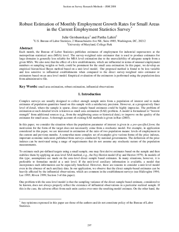The histogram of establishments employment change cannot be described by a nice bell-shaped distribution: it has a spike around zero with very long tails (see Fig.1). The sample is prone to outliers in the sense that there is a high probability that a handful of observations from the tails of the distribution are present in the sample. a. b. Fig.1. a. Histogram of residuals overlayed by the density of the normal distribution with the same first two moments as the estimated moments of the residuals distribution. b. Normal QQ plot of residuals. 3.4 Small Area Estimation in CES a The goal is to estimate the employment trend Rt at a given month t in areas a=1,…,m, where areas are defined by intersection of industry and geography at MSA level within a given State. For area a, the target finite population quantity at month t is given by Rta = ∑ ∑ j∈Pta j∈Pt a y j ,t y j ,t −1 , (3.1) a where Pt is a set of area a population establishments having non-zero employment in both previous (t-1) and current (t) months. Assume the set of finite population observations at month t independent realizations of a random vector of means of (Yt −1 , Yt ) . { ( y j ,t −1 , y j ,t ) | j ∈ Pt (Yt −1 , Yt ) m ∪P ) to be a =1 {( y j ,t −1 } , y j ,t ) | j ∈ Pt a , be independent with the probability distribution Fa and let (θ a t −1 , θ ta ) be a vector of corresponding means . The superpopulation parameter of interest is a function of superpopulation means T ( Fa ) = T (θta−1 ,θta ; Fa ) = a t (Yt −1 , Yt ) having probability distribution F . Denote (θt −1 ,θt ) a vector Let the population measurements in area a, realizations of a random vector } (here, Pt = θta . θta−1 303 (θ a t −1 , θta ) : Section on Survey Research Methods – JSM 2008 The influence function for T defined at F is given by U F ,T ( y j ,t −1 , y j ,t ) = ⎞ θt 1 ⎛ y j ,t −1 ⎟ . ⎜ y j ,t − θt −1 ⎝ θt −1 ⎠ (3.2) As for Tˆ ( FN ) appeared in the formula (2.11), we propose to apply the following survey weighted estimator: θˆ Rˆt = t = θˆ t −1 ∑ ∑ j∈St j∈St w j y j ;t w j y j ;t −1 , (3.3) using sample units from all areas, St = m ∪S a t . This is the same form of the estimator that is normally used for large a =1 areas in the CES. The estimates of means are given by θˆt −1 = ∑ ∑ j∈St w j y j ;t −1 j∈St wj and θˆt = ∑ ∑ j∈St w j y j ;t j∈St wj . The number of population units having non-zero employment in two consecutive months is not known and is estimated by Nˆ a = ∑ j∈S a w j , The sampling fraction is estimated by t n fˆa = a . Nˆ a (3.4) In this application, formula (2.11) reduces to: ES ⎡⎣uˆ wjt | j ∈ Sta ⎦⎤ 1 na ˆ a ˆ ˆ ˆ Rt = Rt + f a ∑ uˆ jt + 1 − f a , na j =1 wa − 1 1 y j ,t − Rˆt y j ,t −1 ; uˆ wjt = ( w j − 1) uˆ jt ; wa = ES ⎡⎣ w j | j ∈ Sta ⎤⎦ . where uˆ jt = ˆ θ ( t −1 ( ) (3.5) ) As displayed on Fig.1, the distribution of uˆ wjt is nearly symmetric; it does not appear to be normal and has a spike near 0 and long tails. A large number of establishments do not have changes in their employment level in a given two consecutive months; others change only by a few employees. This can explain the observed spike. However, there are also establishments that change by quite a large number of employees. The change can be magnified by application of the sampling weights. This economic phenomenon explains the long tails of the distribution. From the above discussion, it is clear that the methods that assume normality or some other standard distribution may result in inefficient estimates. We attend to the problem by assuming the underlying distribution is a mixture of normal distributions and estimating unknown parameters of the distribution using the Bayesian normal mixture model. The MCMC utilizing Gibbs sampler provides a tool for this estimation. At present, we display results of the estimation under the assumption of the mixture of two normal distributions. We also considered the mixture of three and four distributions. The results turned out to be very similar to the two distributions version. On the other hand, the computational burden and monitoring for the convergence proved the approach with greater than two mixture parts to be infeasible in the situation of creating estimates for numerous domains in a short time period. Nevertheless, we formulate the model used in the estimation for the general case of an arbitrary number of mixtures. a Denote xt a a an area-level auxiliary information (at present, we use historical QCEW data: xt =Rt −12 ). We tested the following unit- and area-level models: Model 1 (Mixture of Normal): 304 Section on Survey Research Methods – JSM 2008 uˆ | j ∈ S , C jt = k , μ , σ ~ N ( μ , σ w jt a t 2 k a t ind a t 2 k ) , where μ a t (w = a ( − 1) Rta − Rt − f aU Sa (1 − f a ) ) Rta ~ N ( β xta ,τ 2 ) ind C jt ~ Multi (1, π1 ,..., π K ) π k ~ Dirichlet ( p,..., p ) where a = 1,..., m; j = 1,..., n K is the number of components of the normal mixture; π k is probability to belong to k th component of the mixture, k = 1,..., K ; C jt is class indicator for observation i, which can take the values 1,..., K ; μta is common mean of the mixture distribution for observations from area a; σ k2 is variance parameter of the k th component of the mixture, common for all areas and p is prior probability to belong to component k Model 2 (Normal): uˆ wjt | j ∈ Sta , μta , σ 2 ~ N ( μta , σ 2 ) , where μta = ind ( (w − 1) Rta − Rt − f aU Sa a (1 − f a ) ) Rta ~ N ( β xta ,τ 2 ) ind where a = 1,..., m; j = 1,..., n Model 3 (Fay-Herriot): Rˆta | Rta ~ N ( Rta , σ a2 ) ind Rta ~ N ( β xta ,τ 2 ) ind where a = 1,..., m In models 1 and 2, for the assumed-to-be-known values of wa , ⎛ ( wˆ − 1) ⎜ R a estimates, so that μta = ⎝ a t 1 − Rˆt − fˆa na 1 − fˆ ( a ) na ∑ uˆ j =1 jt Rt , f a , we “plug in” their direct sample based ⎞ ⎟ ⎠ , where wˆ = 1 a na ∑ j∈Sta w j ≠1 w j , na = ∑ j∈S a I w ≠1 , and t j Rˆt and fˆa are given by (3.3) and (3.4), respectively. The method of estimation can be labelled “the empirical hierarchical Bayes”. We used the QCEW historical data to test the approach. We created estimates for September 2006 using the sample drawn from 2005 sampling frame, mimicking the production timeline. Relative growth rates (3.1) were estimated for four States (Alabama, California, Florida, and Pennsylvania). Small areas are defined as metropolitan statistical areas (MSA) at industrial supersector level. In the modeling, each industry was considered separately. The number of areas, m, varied by industries in the four States, ranging from m=12 to m=27. The number of units in the matched sample ranged from 2 to 969 across areas. The resulting estimates were compared to the corresponding true population quantities derived from QCEW. 305 Section on Survey Research Methods – JSM 2008 σ a2 of the direct sample estimator Rˆta . For research purposes, when 2 working with the historical data, we can derive the true variances using all population units. The variances σ a are In model 3, we used true design-based variances assumed to be known in Fay-Herriot model. Of course, we do not have the true values of these variances in real time and would have used the smoothed values of the direct sample estimates of σ a2 . The empirical mean squared error (MSE) was calculated for each industry for the following methods: (1) Model 1 (unit-level, the mixture of two normal distributions); (2) Model 2 (unit-level, the normality assumption); (3) Model 3 (area-level, Fay-Herriot model); (4) the direct sample based estimates of the modified target, Rˆta ; (5) the direct sample based estimates for the original form of the population target, MSE( k )t = ( Rˆta . ) 2 1 m ⎡ a a ⎤ ˆ , − R R 100 ∑ t ( k )t ⎦ m a =1 ⎣ a where Rt is the “true” value obtained from QCEW at month t in area a and industry i (index i is suppressed, for convenience); Rˆ(ak ) t is the estimate of Rta obtained using method k , k = 1,..., 5 . Below are the resulting tables for four states, by industry and overall (column ‘n’ contains the total number of sample units in a given industry): Alabama Industry Construction Manufacturing Durable Goods Manufacturing Nondurable Goods Wholesale Trade Retail Trade Transportation, Warehousing, Utilities Information Finance, Insurance, Real Estate and Rental and Leasing Professional and Business Services Education and Health Services Leisure and Hospitality Other Services Overall n 421 237 109 231 462 Mixture 1.62 0.72 0.37 1.55 0.64 Normal 7.94 1.13 1.22 1.45 1.37 FH 3.82 0.83 0.79 2.83 1.17 Direct (Linear) 21.22 1.57 2.07 11.39 1.42 Direct 45.49 1.18 1.32 12.74 1.42 125 70 2.46 2.00 3.48 1.05 2.23 1.36 4.08 7.80 3.54 5.19 238 659 379 420 181 1.51 0.74 0.38 0.88 25.06 3.16 4.85 2.82 1.28 4.09 37.45 5.68 4.13 3.47 1.46 1.93 21.57 3.80 4.12 2.18 1.88 12.21 86.53 13.04 4.86 2.52 1.98 18.60 90.80 15.80 n 2253 906 801 1410 1819 Mixture 2.45 2.28 22.57 0.94 0.15 Normal 2.98 2.65 28.04 4.68 0.89 FH 3.32 3.24 23.74 4.85 1.30 Direct (Linear) 11.33 6.10 43.91 22.63 2.54 Direct 15.91 9.53 59.92 13.24 4.24 California Industry Construction Manufacturing Durable Goods Manufacturing Nondurable Goods Wholesale Trade Retail Trade 306 Section on Survey Research Methods – JSM 2008 Transportation, Warehousing, Utilities Information Finance, Insurance, Real Estate and Rental and Leasing Professional and Business Services Education and Health Services Leisure and Hospitality Other Services Overall 643 410 6.63 0.97 8.80 1.66 19.24 2.93 35.84 1.85 68.27 7.01 1372 3772 2147 2466 969 0.97 1.44 0.53 1.77 2.98 3.64 1.20 2.59 1.68 2.30 3.59 5.09 4.75 2.64 3.46 2.34 4.08 6.32 19.23 8.73 4.97 4.91 27.85 15.82 9.70 4.91 5.83 5.10 30.56 19.52 n 769 161 86 435 652 Mixture 0.58 1.19 4.93 0.85 0.08 Normal 4.34 1.60 2.99 5.17 0.30 FH 2.97 2.89 4.52 14.20 0.34 Direct (Linear) 8.23 7.42 138.79 44.60 0.36 Direct 7.90 8.14 15.30 24.82 0.51 188 112 1.63 2.10 2.12 4.46 4.23 103.42 14.50 43.46 18.22 112.59 542 1353 723 689 327 0.61 0.49 0.38 1.80 1.14 1.32 0.62 0.75 0.48 2.73 8.17 2.81 1.82 1.39 1.09 3.53 12.07 12.71 4.37 1.29 3.18 17.17 130.62 34.50 6.00 5.08 3.38 13.33 67.39 23.55 n 657 354 215 405 691 Mixture 3.80 0.69 1.80 0.65 0.71 Normal 2.00 1.45 1.63 1.17 0.40 FH 4.69 1.13 1.10 1.27 0.83 Direct (Linear) 19.97 7.35 21.15 11.17 1.76 Direct 24.49 4.82 5.33 5.84 2.99 282 140 20.41 1.62 4.18 1.35 2.21 1.72 25.30 3.24 27.51 3.44 357 1190 939 951 413 1.08 0.95 0.76 7.13 2.64 3.52 1.30 1.40 0.37 2.88 7.73 2.16 8.66 1.15 0.31 2.23 4.22 2.46 6.16 5.68 1.60 11.79 35.67 12.57 17.22 6.72 1.63 10.85 31.98 11.90 Florida Industry Construction Manufacturing Durable Goods Manufacturing Nondurable Goods Wholesale Trade Retail Trade Transportation, Warehousing, Utilities Information Finance, Insurance, Real Estate and Rental and Leasing Professional and Business Services Education and Health Services Leisure and Hospitality Other Services Overall Pennsylvania Industry Construction Manufacturing Durable Goods Manufacturing Nondurable Goods Wholesale Trade Retail Trade Transportation, Warehousing, Utilities Information Finance, Insurance, Real Estate and Rental and Leasing Professional and Business Services Education and Health Services Leisure and Hospitality Other Services Overall 307 Section on Survey Research Methods – JSM 2008 The values of the empirical mean squared errors of the direct sample based estimators for the original and modified targets are of a similar magnitude. All SAE methods considered help to reduce MSE of the direct estimators. Area-level Fay-Herriot estimator works satisfactory except for cases where it is affected by the outlying values (e.g., Florida, Information). Overall, either unit level model has lower MSE than the area level, and in three of the four states considered here, the performance of the mixture model is better. A smaller error in Normal and FH models (compared to the mixture model) for Transportation, Warehousing, Utilities industry of Pennsylvania can be explained by the fact a a that the historical values of the trend ( xt =Rt −12 ) seem to predict well the current trend, yet this predictor receives smaller weight in the mixture model. The model parameters can be adjusted to better account for the degree of reliability of the historical trends. Summary In this paper we proposed a unit level small area model for the case when the finite population quantity of interest has a nonlinear form. The proposed empirical hierarchical Bayesian method that uses a mixture of normal distributions to model the unit level observations has a potential for a useful tool in dealing with influential observations and nonstandard distributions. However, more work is required to overcome practical difficulties associated with the efficient computations in the production environment. One example of the trade-off between efficiency of the procedure and practical considerations is the choice of the number of mixture groups. Larger number of mixture groups may be crucial for the processing time, yet have very little effect on the resulting estimates. Variance of the proposed estimator can be estimated using, for example, the parametric bootstrap method. Work will continue in this direction. References Arora, V., and Lahiri, P. (1997), “On the Superiority of the Bayesian Method Over the BLUP in Small Area Estimation Problems,” Statistica Sinica, 7, 1053–1063 Bureau of Labor Statistics (2004), Chapter 2, “Employment, hours, and earnings from the Establishment survey,” BLS Handbook of Methods. Washington, DC: U.S. Department of Labor. Fay, R.E. and Herriot, (1979). Estimates of Income for Small Places: an Application of James-Stein Procedure to Census Data, Journal of American Statistical Association, 74, 269-277 Folsom, R., Shah, B., Vaish, A. (1999). Substance abuse in states: a methodological report on model based estimates from the 1994–1996 National household survey on drug abuse. Proceedings of the Survey Research Methods Section of the American Statistical Association, pp. 371–375 Hampel, F. (1974). The influence curve and its role in robust estimation, Journal of American Statistical Association, 69, 383–393 Hampel, F.R., Ronchetti, E.M., Rousseeuw, P.J. and Stahel, W.A. (1986). Robust Statistics: the Approach Based on Influence Functions. New-York, John Wiley & Sns, Inc. Hidiroglou, M. (1994) Sampling and Estimation for Establishment Surveys: Stumbling Blocks and Progress. Proceedings of the Survey Research Methods Section of the American Statistical Association, pp. 153-162 Kott, P. (1989). Robust small domain estimation using random effects modelling. Survey Methodology, 15, 1–12 Lee, H. (1995) Outliers in Business Surveys. In Business Survey Methods edited by B. G. Cox, D. A. Binder, B. N. Chinnappa, A. Christianson, M. Colledge, and P. S. Kott, p. 503-526 Pfeffermann, D. and Sverchkov, M. (2007). Small area estimation under informative probability sampling of areas and within the selected areas, Journal of American Statistical Association, 102, 1427-1439 Prasad, N.G.N., Rao, J.N.K. (1999). On robust small area estimation using a simple random e.ects model. Survey Methodology, 25, 67–72 Rao, J.N.K. (2003). Small Area Estimation, New-York, John Wiley & Sons, Inc. Rivest, L.-P. (1999). Stratum jumpers: Can we avoid them? Proceedings of the Survey Research Methods of the American Statistical Association, pp. 64-72. Sarndal, C. E. (1984). Design-Consistent Versus Model-Dependent Estimation for Small Domains, Journal of the American Statistical Association, Vol. 79, No. 387, pp. 624- 631 Sverchkov, M., and Pfeffermann, D. (2004), “Prediction of Finite Population Totals Based on the Sample Distribution,” Survey Methodology, 30, 79–92. Zaslavsky, A.M., Schenker, N. and Belin, T.R. (2001). Downweighting influential clusters in surveys: application to the 1990 post enumeration survey. Journal of the American Statistical Association, 96, 858-869. You, Y. and Rao, J. N. K. (2003). Pseudo hierarchical Bayes small area estimation combining unit level models and survey weights. Journal of Statistical Planning and Inference, 111, 197-208. 308