Comparison of five modelling techniques to predict the spatial distribution and abundance of seabirds

Author's personal copy Biological Conservation 156 (2012) 94–104 Contents lists available at SciVerse ScienceDirect Biological Conservation journal homepage: www.elsevier.com/locate/biocon Comparison of five modelling techniques to predict the spatial distribution and abundance of seabirds Steffen Oppel a,⇑, Ana Meirinho b, Iván Ramírez b, Beth Gardner c, Allan F. O’Connell d, Peter I. Miller e, Maite Louzao f,g a Royal Society for the Protection of Birds, The Lodge, Sandy, Bedfordshire SG19 2DL, UK Sociedade Portuguesa para o Estudo das Aves, Avenida João Crisóstomo N18 4D, 1000-179 Lisboa, Portugal Department of Forestry and Environmental Resources, North Carolina State University, Raleigh, NC 27695, USA d US Geological Survey, Patuxent Wildlife Research Center, Laurel, MD 20708, USA e Plymouth Marine Laboratory, Prospect Place, Plymouth PL1 3DH, UK f UFZ – Helmholtz Centre for Environmental Research, Perlmoserstrasse 15, 04318 Leipzig, Germany g Centre d’Etudes Biologiques de Chizé, CNRS UPR 1934, 79369 Villiers en Bois, France b c a r t i c l e i n f o Article history: Available online 30 December 2011 Keywords: Species distribution model Machine learning Marine protected area Important bird area (IBA) Shearwater Portugal a b s t r a c t Knowledge about the spatial distribution of seabirds at sea is important for conservation. During marine conservation planning, logistical constraints preclude seabird surveys covering the complete area of interest and spatial distribution of seabirds is frequently inferred from predictive statistical models. Increasingly complex models are available to relate the distribution and abundance of pelagic seabirds to environmental variables, but a comparison of their usefulness for delineating protected areas for seabirds is lacking. Here we compare the performance of five modelling techniques (generalised linear models, generalised additive models, Random Forest, boosted regression trees, and maximum entropy) to predict the distribution of Balearic Shearwaters (Puffinus mauretanicus) along the coast of the western Iberian Peninsula. We used ship transect data from 2004 to 2009 and 13 environmental variables to predict occurrence and density, and evaluated predictive performance of all models using spatially segregated test data. Predicted distribution varied among the different models, although predictive performance varied little. An ensemble prediction that combined results from all five techniques was robust and confirmed the existence of marine important bird areas for Balearic Shearwaters in Portugal and Spain. Our predictions suggested additional areas that would be of high priority for conservation and could be proposed as protected areas. Abundance data were extremely difficult to predict, and none of five modelling techniques provided a reliable prediction of spatial patterns. We advocate the use of ensemble modelling that combines the output of several methods to predict the spatial distribution of seabirds, and use these predictions to target separate surveys assessing the abundance of seabirds in areas of regular use. Ó 2011 Elsevier Ltd. All rights reserved. 1. Introduction Marine biodiversity is under increasing human pressure and many species of marine vertebrates have declined over the past decades (Halpern et al., 2008). The decline of many seabird species is directly linked to high mortality at sea due to fisheries bycatch (Croxall and Rothery, 1991; Oro et al., 2004; Weimerskirch, 2002). Reducing mortality of seabirds and other marine biodiversity may be achieved by the designation and enforcement of marine protected areas (Game et al., 2009). Identifying marine areas that are suitable for protection to benefit seabirds requires a thorough understanding of the spatial dis⇑ Corresponding author. Tel.: +44 1767 693452; fax: +44 1767 693211. E-mail addresses: steffen.oppel@rspb.org.uk, steffen.oppel@gmail.com (S. Oppel). 0006-3207/$ - see front matter Ó 2011 Elsevier Ltd. All rights reserved. doi:10.1016/j.biocon.2011.11.013 tribution of seabirds at sea (Louzao et al., 2006a; Lovvorn et al., 2009; Piatt et al., 2006). During the breeding season all seabirds are central place foragers, and the location of important foraging areas at sea are influenced by different factors such as prey availability, foraging ranges and colony sizes of each species (Grecian et al., 2012; Huettmann and Diamond, 2001; Thaxter et al., 2012). Outside the breeding season, however, many species roam widely or migrate long distances, and use distinct areas for stopover (Guilford et al., 2009). Because these foraging areas along migratory routes are equally important for the conservation of seabirds, the identification and protection of those areas is a key priority for seabird conservation (BirdLife International, 2010b; Oppel et al., 2009; Piatt et al., 2006). Determining the spatial distribution of seabirds during the nonbreeding period is difficult because logistical constraints generally Author's personal copy S. Oppel et al. / Biological Conservation 156 (2012) 94–104 limit surveys to subsets of the area of interest. The increasing availability of large-scale remote sensing data, which can be used as environmental predictor variables, makes it possible to use statistical models to predict species distributions over large areas (Elith and Leathwick, 2009; Tremblay et al., 2009). Several statistical modelling techniques have been used to predict the occurrence and abundance of seabirds at sea (Huettmann and Diamond, 2006; Louzao et al., 2009; Nur et al., 2011; Tremblay et al., 2009; Yen et al., 2004). Currently, however, it is not clear how modelling methods differ in their ability to predict species distributions (Elith and Graham, 2009), and which approaches yield the most reliable predictions for seabirds. The number and complexity of modelling techniques used to predict species distributions has increased substantially over the past decades (Hegel et al., 2010), and several comparisons of model performance have been carried out for terrestrial species (e.g., Elith and Graham, 2009; Elith et al., 2006; Segurado and Araújo, 2004). In contrast, the marine environment is less studied and more challenging given its dynamic nature (Ready et al., 2010; Robinson et al., 2011; Wakefield et al., 2009). Furthermore, seabirds are highly mobile species, and their presence at certain locations varies temporally depending on whether an area is used during the breeding season, as a migration stopover, or as moult refuge (Tremblay et al., 2009). A comparison of the performance of different models that predict distributions and abundances of seabirds based on shipboard survey data has to our knowledge only been explored for one coastal species (Yen et al., 2004), yet the bourgeoning interest in the identification of pelagic marine protected areas warrants a comparison of newer distribution modelling techniques. Here we compare the performance of five modelling techniques to predict the occurrence and abundance of a migratory seabird species outside of the breeding season. The Balearic Shearwater (Puffinus mauretanicus) is a critically endangered species that breeds only at the Balearic archipelago in the western Mediterranean, and migrates to the North-East Atlantic after the breeding season (Brooke, 2004). The species suffers from high adult mortality at sea (Oro et al., 2004), and most research efforts have focused on understanding foraging ecology and distribution during the breeding season in the Mediterranean (Bartumeus et al., 2010; Louzao et al., 2006a, 2006b). Marine protected areas are needed for Balearic Shearwaters throughout its range, and although both Spain and Portugal have delineated marine important bird areas (IBAs, Arcos et al., 2009; Ramírez et al., 2008), most of these areas were still not legally protected as of October 2011 (BirdLife International, 2010a). Our model comparison aims to inform seabird conservation managers about the performance of modelling techniques that can be used to predict the spatial distribution and abundance of seabirds for the identification of marine IBAs or protected areas. We tested model predictions against independent data and compared predicted distributions with the locations of existing marine IBAs to evaluate whether our model results agree with IBAs that were identified with a variety of different methods (Ramírez et al., 2008). Thus, we provide information on which modelling techniques are useful for seabirds, and identify areas that may warrant protection to benefit the Balearic Shearwater. 2. Methods 2.1. 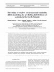Data collection Between December 2004 and April 2009, we conducted shipboard surveys off the coast of Portugal and western Andalusia (Spain) between 36°N and 42°N, and 6°W and 10°W, covering an 95 area of 3497 km2 (Fig. 1). Survey effort was carried out between March and November each year, with fewer surveys from December through February. A total of 1590 h of observations provided data for our analysis, and 84% of the survey effort was in Portuguese waters, 26% in Spanish waters. We used standard European Seabirds at Sea protocols for data collection (Camphuysen and Garthe, 2004; Tasker et al., 1984) on board four similar research vessels. All seabirds in contact with water within 300 m of the survey transect were counted on one side of the ship. All flying seabirds were counted using the ‘snapshot method’, and bird observations were summed over 5 min periods. Based on recorded vessel speed and the nominal width of the survey transect we then calculated the area surveyed (km2), and density of birds as the total number of observed birds divided by the area covered (birds kmÿ2). 2.2. Data processing and exploratory analysis We first binned all observation data into a spatial grid with cell size 4  4 km to match the spatial resolution of remotely sensed environmental data. For each grid cell, we added the number of observed shearwaters during each season and year, and divided this number by the total area surveyed in this cell (hereafter ‘effort’). We were not able to correct density estimates for detectability, as >70% of birds were recorded in flight without an estimated distance to the transect line. Because it is likely that detectability varied as a function of environmental conditions (e.g., sea state, cloud cover), our data provide an index of density rather than a robust estimate of absolute density. Although we recognise that detection of seabirds is imperfect (Ronconi and Burger, 2009), our objective was to evaluate a suite of modelling techniques, all of which used the same data set and therefore suffered from equal bias due to incomplete detection. Every grid cell that had a calculated density >0 received an additional binary detection/non-detection value of ‘1’ (hereafter referred to as ‘presence’), whereas grid cells that were surveyed, but where no Balearic Shearwaters were observed were coded as ‘0’ (hereafter referred to as ‘absence’). We defined ‘seasons’ based on the known phenology of Balearic Shearwaters in the North-East Atlantic (Mouriño et al., 2003; Ruiz and Martí, 2004; Yésou, 2003), and phenological data collected during this project (Ramírez et al., 2008). Balearic Shearwaters breed from late February to late June, and migrate west out of the Mediterranean and then north in the Atlantic between May and July. They moult in the Northeast Atlantic from June to August, and migrate back to the Mediterranean between September and December (Arcos et al., 2009; Mouriño et al., 2003; Yésou, 2003). We therefore considered three seasons: ‘spring’ (January through April, representing mostly non-breeding birds), ‘summer’ (May through August, corresponding to northward migration and moult), and ‘autumn’ (September through December, corresponding to southward migration). Spatial autocorrelation is frequently encountered in ecological data, and not properly accounting for spatial correlation can influence the statistical inference of species distribution models (Dormann, 2007; Dormann et al., 2007; Lichstein et al., 2002). We explored whether there was spatial autocorrelation in Balearic Shearwater distribution and density by calculating Moran’s I (Moran, 1950) and Geary’s C (Geary, 1954) for the 50 nearest neighbouring grid cells using the functions ‘moran.test’ and ‘geary.test’, respectively, in the R-package ‘spdep’. Moran’s I ranges from ÿ1 (perfect dispersion) to +1 (perfect correlation), with values around zero indicative of a random spatial pattern. Geary’s C ranges from 0 to 2, with values < 1 indicative of positive spatial autocorrelation. We found little evidence for spatial autocorrelation in both the distribution (Moran’s I = 0.07 ± 0.05 standard deviation; Geary’s Author's personal copy 96 S. Oppel et al. / Biological Conservation 156 (2012) 94–104 Fig. 1. General map of the study region showing the number of Balearic Shearwaters observed during shipboard surveys between 2005 and 2009. Polygons delimit marine important bird areas identified for Balearic Shearwaters (Ramírez et al., 2008; Arcos et al., 2009). Dashed contour line indicates the edge of the continental shelf (500 m depth contour). Data from the dark grey shaded area served as test data to evaluate the predictive models. C = 0.92 ± 0.05 s.d.) and the density (Moran’s I = 0.02 ± 0.09 s.d.; Geary’s C = 0.98 ± 0.05 s.d.) of Balearic Shearwaters at the spatial scale of our grid cells (16 km2). Hence, we did not specifically incorporate measures to account for spatial autocorrelation in our models, but note that methods to incorporate spatial autocorrelation have recently become available (Hothorn et al., 2011). Our models used latitude and longitude as predictor variables and therefore implicitly included some spatial structure. 2.3. Environmental data To model Balearic Shearwater occurrence and density, we used 13 environmental variables (Table S1) that are either known, or sus- pected, to be correlated with seabird distribution and abundance (Louzao et al., 2006a; Tremblay et al., 2009; Wakefield et al., 2009). Physical variables (distance to coast, mean bathymetry, and bathymetry gradient) were extracted from global bathymetric data (www.ngdc.noaa.gov/mgg/gdas/gd_designagrid.html?dbase =GRDET2) using the cell value nearest to the centroid of each grid cell and were considered invariant throughout the period of our study. Dynamic oceanographic data (sea surface temperature, SST; chlorophyll a concentration, CHL; and sea surface height, SSH) were extracted as monthly averages from Aqua MODIS and Pathfinder AVHRR satellite imagery via NOAA’s BloomWatch data portal (http://coastwatch.pfel.noaa.gov/coastwatch/CWBrowserWW360. jsp), and varied among seasons and years in our study (Table S2). Author's personal copy S. Oppel et al. / Biological Conservation 156 (2012) 94–104 Composite front metrics (density of ocean fronts, and mean distance to nearest major ocean front) were derived from AVHRR satellite imagery (Miller, 2009). Seabird distribution is sometimes uncoupled from current oceanographic conditions measured by variables such as SST and CHL due to time lags between variables that can be measured and the factors (e.g. food availability) that actually attract seabirds (Wakefield et al., 2009). To account for these productivity time lags we integrated SST, CHL, and SSH over a period of three months prior to each season (Louzao et al., 2009; Table S1). We also included the temporal change in SST and CHL as predictor variables, calculated as (maximum SST ÿ minimum SST)  100/maximum SST, with maximum being the highest and minimum the lowest monthly mean SST value in each season. To account for annual anomalies, we included the SST anomaly for each season, calculated as the difference between the average value for a given season and year and the average for that season over a 20-year period in that grid cell. Because seabirds may respond to spatial gradients of oceanographic variables (Louzao et al., 2006a; Tremblay et al., 2009; Wakefield et al., 2009), we also calculated spatial SST and CHL gradients as (maximum value ÿ minimum value)  100/maximum value, with maximum being the highest and minimum the lowest seasonal mean SST or CHL value over a moving 5  5 grid cell window, thus representing 400 km2. This spatial scale was chosen because it provided an excellent fit to observed fronts in the Mediterranean in surveys for Balearic Shearwaters during the breeding season (Louzao et al., 2009; Louzao et al., 2006a). Finally, we used the SSH deviation and composite metrics of ocean fronts in each season as indicators of mesoscale structures that mix additional nutrients up into the surface layer. These structures can sustain higher phytoplankton and zooplankton productivity than surrounding water, and can provide foraging opportunities for seabirds. We did not aim to explore the functional relationships between Balearic Shearwater distribution and environmental variables, but this information is presented in the online supplement (Figs. S1–S17). 2.4. Model construction For marine IBAs, identification criteria depend not only on the presence, but also on the abundance of birds in an area (BirdLife International, 2010b). Hence, useful models must predict both occurrence and abundance. Because of the high mobility of seabirds and imperfect detection at sea, shipboard survey data generally have highly skewed distributions with frequent non-detections (zeros). Such data are difficult to incorporate into standard parametric models (Martin et al., 2005; Sileshi et al., 2009; Warton, 2005). An efficient way to overcome these difficulties is to fit models in a hierarchical fashion (e.g., a ‘hurdle model’), including a component that estimates the occurrence probability, and a subsequent component that estimates the number of individuals given that the species is present (Millar, 2009; Potts and Elith, 2006; Wenger and Freeman, 2008). We adopted that strategy by constructing two separate sets of models, one to predict the presence of Balearic Shearwaters, and one to predict the density of Balearic Shearwaters given their presence in an area. For comparison, we also included a zero-inflated modelling approach to estimate density, which accounts for the large number of non-detections by incorporating the two components described above into one framework (Martin et al., 2005; Potts and Elith, 2006; Warton, 2005). For the occurrence models, we compared five different modelling techniques (for detailed information comparing these methods see Elith et al., 2006; Hegel et al., 2010; Prasad et al., 2006): generalised linear models (GLM; McCullagh and Nelder, 1989), generalised additive models (GAM; Hastie et al., 2001; Wood and Augustin, 2002), and three machine-learning approaches: Random Forest (RF; Breiman, 2001; Cutler et al., 2007), boosted regression 97 trees (BRT; Elith et al., 2008; Friedman, 2002), and maximum entropy (Maxent; Elith et al., 2011; Phillips et al., 2006; Phillips and Dudik, 2008). All models were constructed in R 2.13.0 with the packages ‘mgcv’, ‘gbm’, ‘randomForest’, and ‘dismo’ interfaced with the standalone MaxEnt program v. 3.3.3e. (http://www.cs.princeton.edu/~schapire/maxent/). Maximum entropy is a presence-only modelling approach that uses background samples of the environment rather than absence locations to estimate environmental relationships. We only used those grid cells that were surveyed in a given season and year as background data to facilitate a valid comparison with other models (Elith et al., 2011). Model specifications and software code used to construct the models are available in an online supplement (Appendix S2). We also estimated probability of presence based on an ensemble of all models, as such predictions are often more robust than predictions derived from a single model (Araújo and New, 2007; Marmion et al., 2009; Thuiller et al., 2009). Ensemble predictions were calculated as weighted averages of single-model predictions, with weights assigned to each modelling technique based on its discriminatory power as measured by the area under the receiver-operated characteristic curve (Appendix S2; Araújo and New, 2007; Marmion et al., 2009; Thuiller et al., 2009). For the density model, we used the same modelling techniques as for presence, except for maximum entropy, which is currently not available for modelling non-binary response data. We used the Poisson distribution for the parametric models (the GLM density model, the GAM density model, and the zero-inflated GLM model), because it resulted in better predictions than the negative binomial distribution. Ensemble predictions of density were calculated as above for distribution models, but weighting of models was based on the Pearson correlation coefficient as an indicator. To avoid the influence of extreme observations, we excluded one outlying record of 702 Balearic Shearwaters in a grid cell. We included all environmental predictor variables in each of the modelling approaches. Because inclusion of a large number of variables may lead to over fitting in parametric models, we reduced GLM complexity by sequentially eliminating variables from a full model with all predictors until a minimum AIC was reached. In GAMs, we used the automatic term selection procedure which imposes a penalty to smooth functions and can thus effectively remove terms from the model (Wood and Augustin, 2002). Machine learning approaches are generally robust to the inclusion of a large number of correlated variables (Archer and Kimes, 2008), and we therefore did not reduce the number of variables in these models. To predict the distribution and density for each season and year, we included ‘season’ and ‘year’ as factor variables in each model. In addition, we included latitude and longitude in all models, and the survey effort (in km2) per grid cell in all density models. 2.5. Model evaluation and calibration We divided the survey data into training and test data by setting aside approximately 30% of the surveyed area for spatial evaluation of the models (Araújo and Guisan, 2006; Austin, 2007). All areas north of 39.7°N and south of 38°N were used to construct models (training data), whereas the data in the intermediate sector were used to evaluate the predictive performance of the models (test data, shaded grey in Fig. 1). This division provided sufficient presence data for all seasons in each of the three sectors (>20 grid cells each), and thus allowed for robust model testing. We assessed the performance of distribution models based on the accuracy of predictions for both the training and the independent test data, and report the area under the receiver-operating characteristic curve (AUC) as discrimination performance criteria. AUC ranges from 0 to 1, with values below 0.6 indicating a performance no better than random, values between 0.7–0.9 considered as useful, and values >0.9 as Author's personal copy 98 S. Oppel et al. / Biological Conservation 156 (2012) 94–104 excellent. All model evaluation statistics were calculated using the package ‘PresenceAbsence’ in R 2.11.1 (Appendix S2). Spatial distribution models need to be well calibrated to be useful for predicting beyond the original spatial extent of input observations (Phillips and Elith, 2010; Reineking and Schröder, 2006). In addition to discrimination, which measures a model’s ability to discriminate between presence and absence locations, calibration measures how well the frequency of observations in test data agrees with predicted probabilities of occurrence. To test calibration we used a linear regression of the relative frequency of observed presences over ten bins of predicted probabilities of presence implemented in a binned calibration plot using a custom-made function in R (Phillips and Elith, 2010; Appendix S2). The slope and the intercept of this regression indicate the calibration and the bias of the model, respectively (Phillips and Elith, 2010). In addition, we calculated the point biserial correlation between predicted and observed values, which is sensitive to both discrimination and calibration. For density models, we used the Pearson correlation coefficient and the slope and intercept of a major axis regression of observed over predicted values to evaluate the bias and consistency of model predictions (Pineiro et al., 2008; Potts and Elith, 2006). 2.6. Identification of priority areas for conservation of Balearic Shearwaters To identify priority areas for conservation of Balearic Shearwaters along the W Iberian coast, we used our predicted probabilities of occurrence and the spatial prioritization algorithm ‘Zonation’ (Moilanen, 2007; Moilanen et al., 2005), which has been used successfully in large-scale marine applications (Leathwick et al., 2008). The ‘Zonation’ algorithm ranks areas according to their priority for conservation and is thus ideally suited for conservation planning. The ranking is achieved by sequentially removing grid cells from the study area that have low predicted probabilities of occurrence, and thus the lowest conservation value. The sequential removal also considers proximity of cells to areas of high conservation priority and thus results in a spatially constrained set of priority areas most relevant for conservation (Moilanen, 2007; Moilanen et al., 2005). The approach is designed for the use with multiple species, and marine reserve designation generally requires consideration of multiple species (Ainley et al., 2009; Nur et al., 2011). Here, we only had predicted probabilities of distribution for one species, but we used the predicted distribution in each of our 15 periods (three seasons in each of 5 years) analogous to identifying priority areas for multiple species. We used a simple core-area prioritization in Zonation 2.0 to guarantee the retention of high-quality areas identified in any particular season. We ran the algorithm without boundary quality penalties and a boundary length penalty of 0.1 to retain fewer contiguous areas rather than many small dissociated cells which would be impractical to designate as protected areas. We then compared the most important 10% of the study area retained by the prioritisation algorithm to existing IBAs in Portugal (Ramírez et al., 2008) and Spain (Arcos et al., 2009). The IBAs in Portugal were delineated based on a subset of the data used here, whereas the IBAs in Spain were delineated based on independent data and thus provided a test of the performance of our models. 3. Results 3.1. At-sea surveys We observed 5737 Balearic Shearwaters in 8174 grid cells that were surveyed over the 5 years of study (Fig. 1). On average, 0.7 (±9.8 s.d.) individuals were recorded per km2 of survey effort, but in 91% of grid cells no Balearic Shearwaters were observed. In a further 8% of grid cells only 1–10 birds were observed, and congregations of >100 Balearic Shearwaters were observed on only six occasions throughout the study period (0.07% of surveyed grid cells). 3.2. Performance of distribution models All five modelling techniques had a reasonable ability to discriminate between areas where Balearic Shearwaters were present and absent (all AUC > 0.75, Tables 1 and S3). We found little spatial autocorrelation in model residuals for all models (Moran’s I = 0.03 ± 0.05 s.d., Geary’s C = 0.97 ± 0.05 s.d.). For the training data used to construct the models, the machinelearning approaches RF and BRT provided the best discrimination between areas of presence and absence (highest AUC, Table S3). Maxent was the best-calibrated model, and BRT had the smallest bias. The performance of GLM and GAM was acceptable, but poorer than for the machine-learning approaches when predicting to the data used for model construction (Table S3). By contrast, prediction of independent test data was very similar among the five modelling techniques, with AUC ranging between 0.76 and 0.81 (Table 1). The correlation between predicted presences and observed data also were similar among models (Table 1). The BRT model had the poorest calibration and highest bias, while Maxent showed the best calibration and the GLM had the lowest bias of the five techniques (Table 1). The ensemble prediction showed the best combination of predictive performance and calibration (Table 1). 3.3. Performance of density models As with the occurrence models, performance of density models was very different between training and independent test data. When evaluated for the training data, RF explained 68% of the variation in Balearic Shearwater density, while none of the other models explained >35% of the variation (Table S4). The RF model also showed the highest correlation between observed and predicted density, while the Poisson GLM and GAM showed the best calibration and lowest bias (Table S4). Both GAM and BRT showed relatively high correlation between observed and predicted density, but BRT suffered from poor calibration and relatively large bias. The zero-inflated Poisson and the Poisson GLM explained the least amount of variation (<5%) in the density of Balearic Shearwaters in the training data. None of the models we constructed were able to accurately predict the density of Balearic Shearwaters in the independent test data (Fig. 2, Table 2). In this evaluation, the model performance depended not only on the density model itself, but also on the predictive ability Table 1 Model evaluation and calibration statistics of five modelling techniques and an ensemble predicting the distribution of Balearic Shearwaters in an independent test area. AUC = area under the receiver-operated characteristic curve; COR = point biserial correlation coefficient between observed and predicted values; calibration = slope of regression of observed vs. predicted values; bias = intercept of regression of observed vs. predicted values. See text for description of modelling techniques. Model AUC COR Calibration Bias BRT RF GLM GAM MAX Ensemble 0.80 0.81 0.78 0.76 0.77 0.80 0.25 0.31 0.28 0.24 0.26 0.30 0.03 0.25 0.73 0.36 0.80 0.56 0.18 0.09 0.02 0.07 ÿ0.15 0.02 Author's personal copy 99 S. Oppel et al. / Biological Conservation 156 (2012) 94–104 of the occurrence model of the same technique, because predicted density was the product of predicted probability of presence and predicted density of Balearic Shearwaters for all models except the zero-inflated Poisson model. Neither of the models explained >8% of the variation in recorded density data of Balearic Shearwaters, and the predictive performance of all five models was similarly poor (Table 2). The parametric models (GLM, GAM, and zero-inflated Poisson) had the lowest correlation and explained the least variation. RF had the highest correlation, but was the worst calibrated model with very large bias (Table 2). The ensemble prediction combined the same correlation as the RF model but with substantially smaller bias. In summary, predicting the density of Balearic Shearwaters based on physical and oceanographic data alone was highly unreliable outside the breeding season (Fig. 2). Table 2 Model calibration statistics of five modelling techniques and an ensemble predicting the density (birds/km2) of Balearic Shearwaters in an independent test area. COR = Pearson correlation coefficient between observed and predicted values; rho = Spearman’s rank correlation coefficient; R2, calibration, and bias = coefficient of determination, slope, and intercept of regression of log-transformed observed vs. log-transformed predicted values, respectively. See text for description of modelling techniques. 3.4. Priority areas for conservation of Balearic Shearwaters additional area around Porto has not been previously identified as IBA. The GLM was the only method that identified most of the Spanish IBA‘Entorno marino de las Rías Baixas’ as an area of highest priority for conservation, but in turn considered the two Portuguese IBAs of much lower priority. 6 6 Balearic Shearwater distribution varied among seasons, and seasonal differences were most prominent in the Gulf of Cádiz, with higher predicted probabilities in autumn than in summer (Figs. 3 and 4). Despite their similar performance criteria, the five techniques predicted different distributions of Balearic Shearwaters over the 5 years of our study. Consequently, the areas identified as highest conservation priority for Balearic Shearwaters also differed among techniques (Fig. 5). The areas north of the Spanish–Portuguese border, around Porto, Figuera da Foz, and in the Gulf of Cádiz (Spain) were consistently retained in the most important 10% of the study area. Three of these areas have been identified as marine IBAs by Portugal and Spain (Fig. 1), but an 4 5 3 4 2 3 0 1 2 1 0 -3 -2 -1 0 1 2 3 -3 -2 -1 0 1 2 3 -1 0 1 2 3 0 1 2 3 6 6 POIS 0 0 1 1 2 2 3 3 4 4 5 5 ZIP -2 -1 0 1 2 3 -3 6 6 -3 -2 Ensemble 4 3 2 1 0 0 1 2 3 4 5 GAM 5 observed log density (birds km 2 ) RF 5 BRT -3 -2 -1 0 1 2 3 -3 -2 -1 2 predicted log density (birds km ) Fig. 2. Relationship between observed and predicted density of Balearic Shearwaters in independent test data along the coast of Portugal. BRT: boosted regression trees; RF: Random Forest; ZIP: zero-inflated poisson GLM; POiS: poisson GLM; GAM: generalised additive model; Ensemble: ensemble prediction weighting different models based on the correlation between observed and predicted data. Note that densities were log transformed to enhance display. Model COR Rho R2 Calibration Bias BRT RF ZIP GLM GAM Ensemble 0.12 0.14 0.09 0.03 0.01 0.13 0.26 0.25 0.17 0.17 0.17 0.25 0.08 0.06 0.02 0.02 0.02 0.07 10.5 14.8 6.7 5.1 0.3 14.4 ÿ0.5 ÿ7.7 ÿ0.5 ÿ2.3 ÿ11.7 ÿ0.3 4. Discussion 4.1. Utility of models to identify marine IBAs Our study shows that the choice of modelling method may influence the identification of marine areas for the protection of seabirds. None of the five techniques tested provided superior predictions in all performance criteria, a finding that is consistent with other model comparison studies (Elith and Graham, 2009; Segurado and Araújo, 2004; Syphard and Franklin, 2009). Despite similar predictive performance, the nature of predicted distributions can vary due to different emphasis on and modelled relationships with environmental variables (Elith and Graham, 2009; Ready et al., 2010). In our study, for example, the Maxent and the GLM model had similar predictive performance (Table 1), but would have selected very different areas for the conservation of Balearic Shearwaters (Fig. 5). Because of the uncertainty in choosing a single appropriate technique to identify important areas for seabirds, using a variety of different models and combining them in an ensemble can improve overall prediction (Araújo and New, 2007; Coetzee et al., 2009; Jones-Farrand et al., 2011; Marmion et al., 2009). Our ensemble of five techniques successfully predicted areas of importance for Balearic Shearwaters, including one that had been identified in a different IBA identification project (Arcos et al., 2009). The Spanish IBA ‘Entorno marino de las Rías Baixas’ lies north of the area covered by ship surveys in this project, and thus indicates a reliable prediction of our models to an area that extended beyond the sampling region. Additional independent evidence of the importance and validity of the areas we identified is provided by the recent tracking of Balearic Shearwaters with geolocators and satellite transmitters (T. Guilford & M. Louzao, unpubl. data). In fact, most of the 29 birds tracked with geolocators used at least one of the important areas mentioned above during the non-breeding period and the more fine scale satellite-based tracking data highlights the importance of the IBA Figueira da Foz for a non-breeder. We are therefore confident that the ensemble predictions are robust and we recommend that conservation managers rely on a suite of modelling techniques when trying to identify marine protected areas. Due to recent advances in freely available software, computational challenges for ensemble predictions have decreased considerably (Thuiller, 2003; Thuiller et al., 2009). In contrast to the occurrence models, our density models performed poorly on independent test data (Fig. 2), and we do Author's personal copy 100 S. Oppel et al. / Biological Conservation 156 (2012) 94–104 BRT 42 41 41 40 40 39 39 38 38 37 37 36 36 -10 -9 -8 -7 -6 GLM 42 40 40 39 39 38 38 37 37 36 36 -8 -7 -6 MaxEnt 42 40 40 39 39 38 38 37 37 36 36 -8 -7 -8 -6 -7 -6 0.6 0.4 -9 -8 -7 -6 Ensemble 42 41 -9 -9 GAM -10 41 -10 0.8 42 41 -9 1 -10 41 -10 RF 42 0.2 0 -10 -9 -8 -7 -6 Fig. 3. Predicted distribution of Balearic Shearwater during summer (May–August) 2005–2009 along the coast of southwest Iberia based on five different distribution models and an ensemble prediction across all five models. BRT: boosted regression trees, RF: Random Forest, GLM: generalised linear model, GAM: generalised additive model, MaxEnt: maximum entropy, Ensemble: ensemble prediction across all five models. not recommend their use to estimate whether an area meets the numerical threshold to qualify for a marine IBA (BirdLife International, 2010b). The identification of marine IBAs may benefit from a two-step approach, where the spatial distribution models are used to delineate potential areas where a species occurs regularly, and specific surveys are then conducted in a second step to assess the abundance of target species in those areas. 4.2. Important areas for the conservation of Balearic Shearwaters Our modelling exercise indicated that Balearic Shearwaters use slightly different regions during their northward (May–July) and southward migration (September–December). During summer, shearwaters were present in four marine areas over the continental shelf north of Lisbon (Porto, Figuera da Foz, south of the Berlengas Islands and north of the Spanish–Portuguese border), whereas the Gulf of Cádiz was only used during the southward migration in autumn. The majority of Balearic Shearwaters migrate to the North-East Atlantic before moulting, but some individuals might also moult and stay from June to October over the northern Portuguese continental shelf and in the IBA ‘Rías Baixas’ (Arcos et al., 2009; Mouriño et al., 2003). During autumn migration, birds might forage in additional, seasonally highly productive areas such as the Gulf of Cádiz (García Lafuente and Ruiz, 2007). Our results confirm the high importance of the IBAs ‘Figueira da Foz’, ‘Berlengas’ and ‘Rías Baixas’ (Fig. 1), but suggest that in addition the near-shore waters around Porto are regularly used by Balearic Shearwaters both in summer and in autumn. Low adult survival rates at sea are the main cause for the decline of the Balearic Shearwater population (Louzao et al., 2006b; Oro et al., 2004), and areas that are reliably used by the species during moult and on migration require legal protection to reduce mortality. Our study suggests that the Atlantic coast of Portugal north of Lisbon and extending into Spain serves as an important migratory stopover and/or moulting habitat for Balearic Shearwaters, where protected areas that reduce accidental mortality may Author's personal copy 101 S. Oppel et al. / Biological Conservation 156 (2012) 94–104 BRT 42 41 41 40 40 39 39 38 38 37 37 36 36 -10 -9 -8 -7 -6 GLM 42 40 40 39 39 38 38 37 37 36 36 -8 -7 -6 MaxEnt 42 40 40 39 39 38 38 37 37 36 36 -8 -7 -8 -6 -7 -6 0.6 0.4 -9 -8 -7 -6 Ensemble 42 41 -9 -9 GAM -10 41 -10 0.8 42 41 -9 1 -10 41 -10 RF 42 0.2 0 -10 -9 -8 -7 -6 Fig. 4. Predicted distribution of Balearic Shearwater during autumn (September–December) 2005–2009 along the coast of southwest Iberia based on five different distribution models and an ensemble prediction across all five models. BRT: boosted regression trees, RF: Random Forest, GLM: generalised linear model, GAM: generalised additive model, MaxEnt: maximum entropy, Ensemble: ensemble prediction across all five models. benefit a significant proportion of the species. Further surveys to assess whether the number of Balearic Shearwaters in the nearshore waters around Porto meet marine IBA criteria (BirdLife International, 2010b) would be needed given the socioeconomic costs that may be incurred when marine areas are created for the conservation of seabirds (Adams et al., 2011; Balmford et al., 2004). In addition, the designation of marine reserves would benefit from information on the spatial distribution of multiple species (Ainley et al., 2009; Nur et al., 2011). We therefore recommend integrating the information presented here with similar data for other species, and other stakeholder interests to designate effective marine protected areas for seabirds (Smith et al., 2009). 4.3. Advancing seabird distribution models The vast majority of spatial distribution model literature predicts the distribution of stationary plants or animals in more temporally stable environments. Novel approaches are emerging to model mobile, migratory, or range-shifting species (Elith et al., 2010; Fink et al., 2010; Hothorn et al., 2011; Zurell et al., 2009), but significant challenges still exist in the marine environment, where conditions at a given location are constantly changing (Tremblay et al., 2009; Zipkin et al., 2010). Several unresolved issues exist in seabird distribution models regarding heterogeneity in spatiotemporal scales that may be informed by advances in other environments (Robinson et al., 2011; Schröder, 2008). For example, what time lag exists between the easily measured proxys of primary productivity (e.g., sea surface temperature and chlorophyll a concentration) and foraging conditions that actually attract seabirds? Similarly, is it more useful to model the distribution of pelagic birds separately for each year, using contemporary local environmental measurements, or will predictions that pool observations over several years and use average environmental conditions at a given location provide more robust predictions (Tuanmu et al., 2011)? There may be no single best approach to these issues, and simulations would be useful to thoroughly test Author's personal copy 102 S. Oppel et al. / Biological Conservation 156 (2012) 94–104 BRT 42 41 41 40 40 39 39 38 38 37 37 36 36 -10 -9 -8 -7 -6 GLM 42 -10 41 40 40 39 39 38 38 37 37 36 36 -9 -8 -7 -6 MaxEnt 42 40 40 39 39 38 38 37 37 36 36 -8 top 1% -7 -9 -6 -7 -6 -8 -7 -6 Ensemble 42 41 -9 -8 GAM -10 41 -10 -9 42 41 -10 RF 42 -10 top 5% -9 -8 -7 -6 top 10% Fig. 5. Ranking of marine areas along the coast of southwest Iberia for the conservation of Balearic Shearwaters based on five different distribution models and an ensemble prediction across all five models. BRT: boosted regression trees, RF: Random Forest, GLM: generalised linear model, GAM: generalised additive model, MaxEnt: maximum entropy, Ensemble: ensemble prediction across all five models. Areas were identified using the ‘Zonation’ algorithm, and the colour of shading reflects the priority for conservation (in % of total study area). which combination of temporal aggregation and resolution is most reliable for seabirds at sea. Similar questions exist regarding the choice of environmental predictor variables and modelling techniques. We did not examine the contribution of different variables in this manuscript, and relied on variables commonly used in seabird studies (Tremblay et al., 2009; Wakefield et al., 2009). Although it is well known that different modelling techniques will provide different predictions of the distribution of a species, the causes for these differences are still poorly understood. The most likely reason for differences in the mapped predictions for occurrence between models are differences in the functions fitted by each technique (Elith and Graham, 2009). Different predictor variables and varying levels of complexities in the fitted functions (Figs. S1–S17) are likely to explain differences between the machine-learning and the parametric modelling approaches in our study (Dormann et al., 2008; Syphard and Franklin, 2009), but a detailed analysis of the specific model differences is beyond the scope of this contribution. The machine-learning methods RF, BRT, and Maxent provided excellent discrimination between areas where Balearic Shearwaters were present and absent. However, when used on spatially independent test data, the predictive performance of those three models was only marginally better than GLM and GAM approaches, suggesting that the machine learning methods suffer proportionally more from over fitting than parametric models (Dormann et al., 2008; Hastie et al., 2001). A similar pattern emerged for the density models, where RF showed good performance on the training data, but equally poor performance as other models when predicting shearwater density in independent test data. Many seabird surveys yield only brief temporal windows into the spatial distribution of seabirds, and many recorded absences may therefore be considered as false absences, because seabirds may have been present in that area at a time when the surveyors were not. Such methodological absences reduce the power of spatial distribution and abundance models (Lobo et al., 2010; Martin et al., 2005), and create uncertainty when models are evaluated. Therefore, Lobo et al. (2010) suggested removing absences that are identical or close to observed presences in environmental space from the training data to remove the potential effect of false absences. False absences may also have contributed to the poor performance of our density models, as the hurdle model approach that we employed assumes that zero observations reflect true absence (Risk et al., 2011). However, even when predicted to only the presence fraction of independent test data our density models showed weak correlation with observed densities. More sophisticated models that simultaneously model the observation and process uncertainty and can thus account for imperfect detection may provide better estimates of spatial abundance patterns in the future (Dail and Madsen, 2011; Hutchinson et al., 2011; Warton and Shepherd, 2010). Acknowledgements Data collection for this project started with LIFE 04NAT/PT/ 000213 funding by the European Union, and we thank IPIMAR (Instituto de Investigação das Pescas e do Mar) and the Instituto Hidrográfico Português for subsequent support in data collection. We thank all research institutions that allowed observers onboard the survey vessels, and all observers and volunteers of the LIFE project. M.L. was funded by a Marie Curie Individual Fellowship (PIEFGA-2008-220063). G. Buchanan, A. Marcer and R. Hijmans assisted with maximum entropy modelling. The manuscript benefited from thoughtful comments by B. Best, G. Humphries, J. M. Arcos, R. A. Ronconi, E. Owen, N. Nur, and two anonymous reviewers. Appendix A. Supplementary material Supplementary data associated with this article can be found, in the online version, at doi:10.1016/j.biocon.2011.11.013. Author's personal copy S. Oppel et al. / Biological Conservation 156 (2012) 94–104 References Adams, V.M., Mills, M., Jupiter, S.D., Pressey, R.L., 2011. Improving social acceptability of marine protected area networks: a method for estimating opportunity costs to multiple gear types in both fished and currently unfished areas. Biological Conservation 144, 350–361. Ainley, D.G., Dugger, K.D., Ford, R.G., Pierce, S.D., Reese, D.C., Brodeur, R.D., Tynan, C.T., Barth, J.A., 2009. Association of predators and prey at frontal features in the California current: competition, facilitation, and co-occurrence. Marine Ecology Progress Series 389, 271–294. Araújo, M.B., Guisan, A., 2006. Five (or so) challenges for species distribution modelling. Journal of Biogeography 33, 1677–1688. Araújo, M.B., New, M., 2007. Ensemble forecasting of species distributions. Trends in Ecology & Evolution 22, 42–47. Archer, K.J., Kimes, R.V., 2008. Empirical characterization of random forest variable importance measures. Computational Statistics and Data Analysis 52, 2249– 2260. Arcos, J.M., Bécares, J., Rodríguez, B., Ruiz, A., 2009. Áreas Importantes para la Conservación de las Aves marinas en España. Sociedad Española de Ornitología (SEO/BirdLife), Madrid, Spain. Austin, M., 2007. Species distribution models and ecological theory: a critical assessment and some possible new approaches. Ecological Modelling 200, 1– 19. Balmford, A., Gravestock, P., Hockley, N., McClean, C.J., Roberts, C.M., 2004. The worldwide costs of marine protected areas. Proceedings of the National Academy of Sciences of the United States of America 101, 9694–9697. Bartumeus, F., Giuggioli, L., Louzao, M., Bretagnolle, V., Oro, D., Levin, S.A., 2010. Fishery discards impact on seabird movement patterns at regional scales. Current Biology 20, 215–222. BirdLife International, 2010a. Marine IBAs in the European Union. BirdLife International, Brussels, Belgium. BirdLife International, 2010b. Marine Important Bird Areas Toolkit: Standardised Techniques for Identifying Priority Sites for the Conservation of Seabirds At-Sea. BirdLife International, Cambridge, UK. Breiman, L., 2001. Random forests. Machine Learning 45, 5–32. Brooke, M., 2004. Albatrosses and Petrels Across the World. Oxford University Press, USA. Camphuysen, K.C.J., Garthe, S., 2004. Recording foraging seabirds at sea: standardised recording and coding of foraging behaviour and multi-species foraging associations. Atlantic Seabirds 6, 1–32. Coetzee, B.W.T., Robertson, M.P., Erasmus, B.F.N., van Rensburg, B.J., Thuiller, W., 2009. Ensemble models predict Important Bird Areas in southern Africa will become less effective for conserving endemic birds under climate change. Global Ecology and Biogeography 18, 701–710. Croxall, J., Rothery, P., 1991. Population regulation of seabirds: implications of their demography for conservation. In: Perrins, C.M., Lebreton, J.D., Hirons, G.M. (Eds.), Bird Population Studies, Relevance to Conservation and Management. Oxford University Press, Oxford, UK, pp. 272–296. Cutler, D.R., Edwards, T.C., Beard, K.H., Cutler, A., Hess, K.T., Gibson, J., Lawler, J.J., 2007. Random forests for classification in ecology. Ecology 88, 2783–2792. Dail, D., Madsen, L., 2011. Models for estimating abundance from repeated counts of an open metapopulation. Biometrics 67, 577–578. Dormann, C.F., 2007. Effects of incorporating spatial autocorrelation into the analysis of species distribution data. Global Ecology and Biogeography 16, 129– 138. Dormann, C.F., McPherson, J.M., Araújo, M.B., Bivand, R., Bolliger, J., Carl, G., Davies, R.G., Hirzel, A., Jetz, W., Kissling, W.D., 2007. Methods to account for spatial autocorrelation in the analysis of species distributional data: a review. Ecography 30, 609–628. Dormann, C.F., Purschke, O., Marquez, J.R.G., Lautenbach, S., Schröder, B., 2008. Components of uncertainty in species distribution analysis: a case study of the Great Grey Shrike. Ecology 89, 3371–3386. Elith, J., Graham, C.H., 2009. Do they? How do they? WHY do they differ? On finding reasons for differing performances of species distribution models. Ecography 32, 66–77. Elith, J., Graham, C.H., Anderson, R.P., Dudik, M., Ferrier, S., Guisan, A., Hijmans, R.J., Huettmann, F., Leathwick, J.R., Lehmann, A., Li, J., Lohmann, L.G., Loiselle, B.A., Manion, G., Moritz, C., Nakamura, M., Nakazawa, Y., Overton, J.M., Peterson, A.T., Phillips, S.J., Richardson, K., Scachetti-Pereira, R., Schapire, R.E., Soberon, J., Williams, S., Wisz, M.S., Zimmermann, N.E., 2006. Novel methods improve prediction of species’ distributions from occurrence data. Ecography 29, 129– 151. Elith, J., Kearney, M., Phillips, S., 2010. The art of modelling range-shifting species. Methods in Ecology and Evolution 1, 330–342. Elith, J., Leathwick, J.R., 2009. Species distribution models: ecological explanation and prediction across space and time. Annual Review of Ecology, Evolution, and Systematics 40, 677–697. Elith, J., Leathwick, J.R., Hastie, T., 2008. A working guide to boosted regression trees. Journal of Animal Ecology 77, 802–813. Elith, J., Phillips, S.J., Hastie, T., Dudík, M., Chee, Y.E., Yates, C.J., 2011. A statistical explanation of MaxEnt for ecologists. Diversity and Distributions 17, 43–57. Fink, D., Hochachka, W.M., Zuckerberg, B., Winkler, D.W., Shaby, B., Munson, M.A., Hooker, G., Riedewald, M., Sheldon, D., Kelling, S., 2010. Spatiotemporal exploratory models for broad-scale survey data. Ecological Applications 20, 2131–2147. 103 Friedman, J.H., 2002. Stochastic gradient boosting. Computational Statistics & Data Analysis 38, 367–378. Game, E.T., Grantham, H.S., Hobday, A.J., Pressey, R.L., Lombard, A.T., Beckley, L.E., Gjerde, K., Bustamante, R., Possingham, H.P., Richardson, A.J., 2009. Pelagic protected areas: the missing dimension in ocean conservation. Trends in Ecology & Evolution 24, 360–369. García Lafuente, J., Ruiz, J., 2007. The Gulf of Cádiz pelagic ecosystem: a review. Progress in Oceanography 74, 228–251. Geary, R.C., 1954. The contiguity ratio and statistical mapping. Incorporated Statistician 5, 115–146. Grecian, W.J., Witt, M.J., Attrill, M.J., Bearhop, S., Godley, B.J., Grémillet, D., Hamer, K.C., Votier, S.C., 2012. A novel projection technique to identify important at-sea areas for seabird conservation: an example using Northern gannets breeding in the North East Atlantic. Biological Conservation this issue. Guilford, T., Meade, J., Willis, J., Phillips, R.A., Boyle, D., Roberts, S., Collett, M., Freeman, R., Perrins, C.M., 2009. Migration and stopover in a small pelagic seabird, the Manx shearwater Puffinus puffinus: insights from machine learning. Proceedings of the Royal Society B 276, 1215–1223. Halpern, B.S., Walbridge, S., Selkoe, K.A., Kappel, C.V., Micheli, F., D’Agrosa, C., Bruno, J.F., Casey, K.S., Ebert, C., Fox, H.E., Fujita, R., Heinemann, D., Lenihan, H.S., Madin, E.M.P., Perry, M.T., Selig, E.R., Spalding, M., Steneck, R., Watson, R., 2008. A global map of human impact on marine ecosystems. Science 319, 948–952. Hastie, T., Tibshirani, R., Friedman, J.H., 2001. The Elements of Statistical Learning: Data Mining, Inference, and Prediction. Springer, New York, NJ. Hegel, T.M., Cushman, S.A., Evans, J., Huettmann, F., 2010. Current state of the art for statistical modelling of species distributions. In: Cushman, S., Huettmann, F. (Eds.), Spatial Complexity, Informatics, and Wildlife Conservation. Springer, Tokyo, pp. 273–311. Hothorn, T., Müller, J., Schröder, B., Kneib, T., Brandl, R., 2011. Decomposing environmental, spatial, and spatiotemporal components of species distributions. Ecological Monographs 81, 329–347. Huettmann, F., Diamond, A., 2006. Large-scale effects on the spatial distribution of seabirds in the Northwest Atlantic. Landscape Ecology 21, 1089–1108. Huettmann, F., Diamond, A.W., 2001. Seabird colony locations and environmental determination of seabird distribution: a spatially explicit breeding seabird model for the Northwest Atlantic. Ecological Modelling 141, 261–298. Hutchinson, R.A., Liu, L.-P., Dietterich, T.G., 2011. Incorporating boosted regression trees into ecological latent variable models. In: 25th AAAI Conference on Artificial Intelligence. Association for the Advancement of Artificial Intelligence, San Francisco, CA. Jones-Farrand, D.T., Fearer, T.M., Thogmartin, W.E., Iii, F.R.T., Nelson, M.D., Tirpak, J.M., 2011. Comparison of statistical and theoretical habitat models for conservation planning: the benefit of ensemble prediction. Ecological Applications 21, 2269–2282. Leathwick, J., Moilanen, A., Francis, M., Elith, J., Taylor, P., Julian, K., Hastie, T., Duffy, C., 2008. Novel methods for the design and evaluation of marine protected areas in offshore waters. Conservation Letters 1, 91–102. Lichstein, J., Simons, T., Shriner, S., Franzreb, K., 2002. Spatial autocorrelation and autoregressive models in ecology. Ecological Monographs 72, 445–463. Lobo, J.M., Jiménez-Valverde, A., Hortal, J., 2010. The uncertain nature of absences and their importance in species distribution modelling. Ecography 33, 103–114. Louzao, M., Becares, J., Rodriguez, B., Hyrenbach, K.D., Ruiz, A., Arcos, J.M., 2009. Combining vessel-based surveys and tracking data to identify key marine areas for seabirds. Marine Ecology Progress Series 391, 183–197. Louzao, M., Hyrenbach, K., Arcos, J., Abelló, P., de Sola, L., Oro, D., 2006a. Oceanographic habitat of an endangered Mediterranean procellariiform: implications for marine protected areas. Ecological Applications 16, 1683–1695. Louzao, M., Igual, J., McMinn, M., Aguilar, J., Triay, R., Oro, D., 2006b. Small pelagic fish, trawling discards and breeding performance of the critically endangered Balearic shearwater: improving conservation diagnosis. Marine Ecology Progress Series 318, 247–254. Lovvorn, J.R., Grebmeier, J.M., Cooper, L.W., Bump, J.K., Richman, S.E., 2009. Modeling marine protected areas for threatened eiders in a climatically changing Bering Sea. Ecological Applications 19, 1596–1613. Marmion, M., Parviainen, M., Luoto, M., Heikkinen, R.K., Thuiller, W., 2009. Evaluation of consensus methods in predictive species distribution modelling. Diversity and Distributions 15, 59–69. Martin, T.G., Wintle, B.A., Rhodes, J.R., Kuhnert, P.M., Field, S.A., Low-Choy, S.J., Tyre, A.J., Possingham, H.P., 2005. Zero tolerance ecology: improving ecological inference by modelling the source of zero observations. Ecology Letters 8, 1235–1246. McCullagh, P., Nelder, J.A., 1989. Generalized Linear Models. Chapman and Hall, Washington, DC, USA. Millar, R.B., 2009. Comparison of hierarchical Bayesian models for overdispersed count data using DIC and Bayes’ factors. Biometrics 65, 962–969. Miller, P., 2009. Composite front maps for improved visibility of dynamic seasurface features on cloudy SeaWiFS and AVHRR data. Journal of Marine Systems 78, 327–336. Moilanen, A., 2007. Landscape zonation, benefit functions and target-based planning: unifying reserve selection strategies. Biological Conservation 134, 571–579. Moilanen, A., Franco, A.M.A., Early, R.I., Fox, R., Wintle, B., Thomas, C.D., 2005. Prioritizing multiple-use landscapes for conservation: methods for large multispecies planning problems. Proceedings of the Royal Society B: Biological Sciences 272, 1885–1891. Author's personal copy 104 S. Oppel et al. / Biological Conservation 156 (2012) 94–104 Moran, P.A.P., 1950. Notes on continuous stochastic phenomena. Biometrika 37, 17. Mouriño, J., Arcos, F., Salvadores, R., Sandoval, A., Vidal, C., 2003. Status of the Balearic shearwater (Puffinus mauretanicus) on Galician coast (NW Iberian Peninsula). Scientia Marina 67, 135–142. Nur, N., Jahncke, J., Herzog, M.P., Howar, J., Hyrenbach, K.D., Zamon, J.E., Ainley, D.G., Wiens, J.A., Morgan, K., Ballance, L.T., Stralberg, D., 2011. Where the wild things are: predicting hotspots of seabird aggregations in the California current system. Ecological Applications 21, 2241–2257. Oppel, S., Dickson, D.L., Powell, A.N., 2009. International importance of the eastern Chukchi Sea as a staging area for migrating King Eiders. Polar Biology 32, 775– 783. Oro, D., Aguilar, J.S., Igual, J.M., Louzao, M., 2004. Modelling demography and extinction risk in the endangered Balearic shearwater. Biological Conservation 116, 93–102. Phillips, S.J., Anderson, R.P., Schapire, R.E., 2006. Maximum entropy modeling of species geographic distributions. Ecological Modelling 190, 231–259. Phillips, S.J., Dudik, M., 2008. Modeling of species distributions with Maxent: new extensions and a comprehensive evaluation. Ecography 31, 161–175. Phillips, S.J., Elith, J., 2010. POC plots: calibrating species distribution models with presence-only data. Ecology 91, 2476–2484. Piatt, J.F., Wetzel, J., Bell, K., DeGange, A.R., Balogh, G.R., Drew, G.S., Geernaert, T., Ladd, C., Byrd, G.V., 2006. Predictable hotspots and foraging habitat of the endangered short-tailed albatross (Phoebastria albatrus) in the North Pacific: Implications for conservation. Deep Sea Research Part II 53, 387–398. Pineiro, G., Perelman, S., Guerschman, J.P., Paruelo, J.M., 2008. How to evaluate models: observed vs. predicted or predicted vs. observed? Ecological Modelling 216, 316–322. Potts, J.M., Elith, J., 2006. Comparing species abundance models. Ecological Modelling 199, 153–163. Prasad, A.M., Iverson, L.R., Liaw, A., 2006. Newer classification and regression tree techniques: bagging and random forests for ecological prediction. Ecosystems 9, 181–199. Ramírez, I., Geraldes, P., Meirinho, A., Amorim, P., Paiva, V.H., 2008. Areas Importantes Para as Aves Marinhas em Portugal. Sociedade Portuguesa para o Estudo das Aves, Lisbon, Portugal. Ready, J., Kaschner, K., South, A.B., Eastwood, P.D., Rees, T., Rius, J., Agbayani, E., Kullander, S., Froese, R., 2010. Predicting the distributions of marine organisms at the global scale. Ecological Modelling 221, 467–478. Reineking, B., Schröder, B., 2006. Constrain to perform: regularization of habitat models. Ecological Modelling 193, 675–690. Risk, B.B., de Valpine, P., Beissinger, S.R., 2011. A robust-design formulation of the incidence function model of metapopulation dynamics applied to two species of rails. Ecology 92, 462–474. Robinson, L.M., Elith, J., Hobday, A.J., Pearson, R.G., Kendall, B.E., Possingham, H.P., Richardson, A.J., 2011. Pushing the limits in marine species distribution modelling: lessons from the land present challenges and opportunities. Global Ecology and Biogeography 20, 789–802. Ronconi, R.A., Burger, A.E., 2009. Estimating seabird densities from vessel transects: distance sampling and implications for strip transects. Aquatic Biology 4, 297– 309. Ruiz, A., Martí, R. (Eds.), 2004. La pardela Balear. SEO/BirdLife-Conselleria de Medi Ambient del Govern de les Iles Balears, Madrid, Spain. Schröder, B., 2008. Challenges of species distribution modeling belowground. Journal of Plant Nutrition and Soil Science 171, 325–337. Segurado, P., Araújo, M.B., 2004. An evaluation of methods for modelling species distributions. Journal of Biogeography 31, 1555–1568. Sileshi, G., Hailu, G., Nyadzi, G.I., 2009. Traditional occupancy-abundance models are inadequate for zero-inflated ecological count data. Ecological Modelling 220, 1764–1775. Smith, R.J., Eastwood, P.D., Ota, Y., Rogers, S.I., 2009. Developing best practice for using Marxan to locate marine protected areas in European waters. ICES Journal of Marine Science 66, 188–194. Syphard, A.D., Franklin, J., 2009. Differences in spatial predictions among species distribution modeling methods vary with species traits and environmental predictors. Ecography 32, 907–918. Tasker, M.L., Jones, P.H., Dixon, T., Blake, B.F., 1984. Counting seabirds at sea from ships: a review of methods employed and a suggestion for a standardized approach. Auk 101, 567–577. Thaxter, C., Lascelles, B., Sugar, K., Cook, A.S., Roos, S., Bolton, M., Langston, R., Burton, N.H., 2012. Seabird foraging ranges as a preliminary tool for identifying candidate Marine Protected Areas. Biological Conservation, this issue. Thuiller, W., 2003. BIOMOD – optimizing predictions of species distributions and projecting potential future shifts under global change. Global Change Biology 9, 1353–1362. Thuiller, W., Lafourcade, B., Engler, R., Araujo, M.B., 2009. BIOMOD – a platform for ensemble forecasting of species distributions. Ecography 32, 369–373. Tremblay, Y., Bertrand, S., Henry, R.W., Kappes, M.A., Costa, D.P., Shaffer, S.A., 2009. Analytical approaches to investigating seabird-environment interactions: a review. Marine Ecology Progress Series 391, 153–163. Tuanmu, M.-N., Viña, A., Roloff, G.J., Liu, W., Ouyang, Z., Zhang, H., Liu, J., 2011. Temporal transferability of wildlife habitat models: implications for habitat monitoring. Journal of Biogeography 38, 1510–1523. Wakefield, E.D., Phillips, R.A., Matthiopoulos, J., 2009. Quantifying habitat use and preferences of pelagic seabirds using individual movement data: a review. Marine Ecology Progress Series 391, 165–182. Warton, D.I., 2005. Many zeros does not mean zero inflation: comparing the goodness-of-fit of parametric models to multivariate abundance data. Environmetrics 16, 275–289. Warton, D.I., Shepherd, L.C., 2010. Poisson point process models solve the ‘‘pseudoabsence problem’’ for presence-only data in ecology. Annals of Applied Statistics. Weimerskirch, H., 2002. Seabird demography and its relationship with the marine environment. In: Schreiber, E.A., Burger, J. (Eds.), Biology of Marine Birds. CRC Press, Boca Raton, Florida, pp. 115–135. Wenger, S.J., Freeman, M.C., 2008. Estimating species occurrence, abundance, and detection probability using zero-inflated distributions. Ecology 89, 2953–2959. Wood, S.N., Augustin, N.H., 2002. GAMs with integrated model selection using penalized regression splines and applications to environmental modelling. Ecological Modelling 157, 157–177. Yen, P.P.W., Huettmann, F., Cooke, F., 2004. A large-scale model for the at-sea distribution and abundance of Marbled Murrelets (Brachyramphus marmoratus) during the breeding season in coastal British Columbia, Canada. Ecological Modelling 171, 395–413. Yésou, P., 2003. Recent changes in the summer distribution of the Balearic shearwater Puffinus mauretanicus off western France. Scientia Marina, 67. Zipkin, E., Gardner, B., Gilbert, A., O’Connell, A., Royle, J., Silverman, E., 2010. Distribution patterns of wintering sea ducks in relation to the North Atlantic Oscillation and local environmental characteristics. Oecologia 163, 893–902. Zurell, D., Jeltsch, F., Dormann, C.F., Schröder, B., 2009. Static species distribution models in dynamically changing systems: how good can predictions really be? Ecography 32, 733–744.