Extremes
DOI 10.1007/s10687-016-0261-5
Mean-of-order p reduced-bias extreme value index
estimation under a third-order framework
Frederico Caeiro1 · M. Ivette Gomes2 ·
Jan Beirlant3,4 · Tertius de Wet5
Received: 5 May 2015 / Revised: 6 June 2016 / Accepted: 8 June 2016
© Springer Science+Business Media New York 2016
Abstract Reduced-bias versions of a very simple generalization of the ‘classical’
Hill estimator of a positive extreme value index (EVI) are put forward. The Hill estimator can be regarded as the logarithm of the mean-of-order-0 of a certain set of
statistics. Instead of such a geometric mean, it is sensible to consider the mean-oforder-p (MOP) of those statistics, with p real. Under a third-order framework, the
asymptotic behaviour of the MOP, optimal MOP and associated reduced-bias classes
of EVI-estimators is derived. Information on the dominant non-null asymptotic bias
is also provided so that we can deal with an asymptotic comparison at optimal levels of some of those classes. Large-scale Monte-Carlo simulation experiments are
undertaken to provide finite sample comparisons.
� Frederico Caeiro
fac@fct.unl.pt
M. Ivette Gomes
ivette.gomes@fc.ul.pt
Jan Beirlant
jan.beirlant@kuleuven.be
Tertius de Wet
tdewet@sun.ac.za
1
CMA and DM, FCT, Universidade Nova de Lisboa, Lisbon, Portugal
2
CEAUL and DEIO, FCUL, Universidade de Lisboa, Lisbon, Portugal
3
KU Leuven, Leuven, Belgium
4
University of the Free State, Bloemfontein, South Africa
5
Stellenbosch University, Stellenbosch, South Africa
�F. Caeiro et al.
Keywords Bias estimation · Heavy tails · Optimal levels · Semi-parametric
reduced-bias estimation · Statistics of extremes
AMS 2000 Subject Classifications Primary 62G32 · Secondary 65C05
1 Introduction
Given a sample of size n of independent and identically distributed random variables
(RVs), X1 , . . . , Xn , with a common cumulative distribution function (CDF) F , let
us denote the associated ascending order statistics by X1:n ≤ · · · ≤ Xn:n . Let us
further assume that there exist sequences of real constants {an > 0} and {bn ∈ R}
such that (Xn:n − bn ) /an converges in distribution to a non-degenerate RV. Then, as
first proved in Gnedenko (1943), the limiting CDF is necessarily of the type of the
general extreme value (EV) CDF, given by
�
exp(−(1 + ξ x)−1/ξ ), 1 + ξ x > 0, if ξ � = 0,
EVξ (x) =
(1.1)
exp(− exp(−x)), x ∈ R,
if ξ = 0.
The CDF F is then
� said� to belong to the max-domain of attraction of EVξ and the
notation F ∈ DM EVξ is used. The parameter ξ in Eq. 1.1 is the extreme value
index (EVI) for maxima, the primary parameter of large extreme events. This EVI
measures the heaviness of the right tail-function, F (x) := 1 − F (x), and the heavier
the right tail, the larger ξ is.
Let us further use the notation Ra for the class of regularly varying functions at
infinity, with an index of regular variation a ∈ R, i.e. positive measurable functions
g(·) such that for all x > 0, g(tx)/g(t) → x a , as t → ∞ (see Bingham et al.
(1987), for details on regular variation). In this article we work with Pareto-type
underlying parents, with a positive EVI, or equivalently, right tail-functions such that
F (x) = x −α L(x), α = 1/ξ > 0, with L ∈ R0 . These heavy-tailed models are
quite common in many areas of application, such as biostatistics, computer science,
finance, insurance and social sciences, among others.
For Pareto-type models, the Hill (H) estimator (Hill 1975) is the classical
estimator, which is the average of the log-excesses of the k top data,
V := {Vik := ln Xn−i+1:n − ln Xn−k:n ,
1 ≤ i ≤ k < n} ,
(1.2)
being thus the logarithm of the geometric mean (or mean-of-order-0) of
U := exp(V) = {Uik := Xn−i+1:n /Xn−k:n , 1 ≤ i ≤ k < n} .
(1.3)
Brilhante et al. (2013) considered the mean-of-order-p (MOP) of U, in Eq. 1.3,
with p ≥ 0. Here, we more generally consider p ∈ R, and the class of MOP
EVI-estimators,
⎧
−1
k
⎪
⎪
p
1
1
⎪
⎪
U
,
if p < 1/ξ, p � = 0,
1
−
⎨p
ik
k
i=1
Hk (p) :=
(1.4)
1/k
⎪
k
k
�
⎪
1
⎪
⎪
Vik =: Hk , if p = 0,
=k
Uik
⎩ ln
i=1
i=1
�Mean-of-order p reduced-bias extreme value index estimation...
with Hk ≡ Hk (0), the Hill EVI-estimator. This class of MOP EVI-estimators depends
on the tuning parameter p ∈ R, and can be consistent for any real p < 1/ξ . It is
indeed a highly flexible class of EVI-estimators, but it is not asymptotically unbiased
for the moderate k-values leading to minimum mean square error (MSE).
For technical simplicity, let us consider the Hall-Welsh class of models (Hall and
Welsh 1985), i.e. let us assume that, with U (t) := F ← (1 − 1/t), t ≥ 1, the tail
quantile function, and using the notation F ← (t) := inf{x : F (x) ≥ t}, 0 ≤ t ≤ 1,
�
�
U (t) = C t ξ 1 + A(t)/ρ + o(t ρ ) ,
A(t) := ξβt ρ ,
(1.5)
as t → ∞, C > 0, ξ > 0, ρ < 0 and β � = 0.
Then, as noticed in Brilhante et al. (2014), there is an optimal value for p given by
�
�
�
√ �
pM := ϕρ /ξ, with ϕρ := 1−ρ/2− ρ 2 − 4ρ + 2 2 ∈ 0, 1 − 2/2 , (1.6)
which maximizes the asymptotic efficiency of the class of estimators in Eq. 1.4 with
respect to the Hill estimator, leading to an optimal MOP class, Hk := Hk (pM ).
From Brilhante et al. (2013) (see also, de Haan and Peng (1998),
√ for p = 0), it
follows that under Eq. 1.5, for 0 ≤ p < 1/(2ξ ), λ(1)
:=
lim
k A(n/k) finite,
n→∞
A
�
�
and the notation N μ, σ 2 indicating a normal RV with mean value μ and variance
σ 2 , we have that,
�
�
√
2 (1−pξ )2
d
1−pξ
(1)
2
(1)
2
, bH(p)
b
,
σ
= 1−ρ−pξ
k (Hk (p) − ξ ) −→ N λ(1)
, σH(p)
= ξ 1−2pξ
.
A
H(p)
H(p)
n→∞
(1.7)
It is easy to check that the result in Eq. 1.7 also holds for p < 0. Hence the
MOP class in Eq. 1.4 has a dominant component of asymptotic bias given by
A(n/k)(1 − pξ )/(1 − ρ − pξ ) = ξβ(n/k)ρ (1 − pξ )/(1 − ρ − pξ ). We thus find
that RVs of the type
RBk (p, β, ρ, φ) := Hk (p) 1 −
β(1 − φ) � n �ρ
,
1−ρ−φ k
(1.8)
will lead to reduced bias (RB) estimators, replacing φ by estimators of pξ or of ϕρ =
pM ξ . Gomes et al. (2015) introduced the partially RB MOP class of EVI-estimators,
�
�
(1.9)
RBk (p) ≡ RBk (p, β̂, ρ̂) := RBk p, β̂, ρ̂, ϕρ̂ ,
also dependent on a tuning parameter p and on (β̂, ρ̂), an adequate estimator of
(β, ρ) in Eq. 1.5. In this paper we further consider
�
�
(1.10)
RBk (p) ≡ RBk (p, β̂, ρ̂) := RBk p, β̂, ρ̂, pHk (p) .
Both in Eqs. 1.9 and 1.10, we can consider p replaced by an estimator of the optimal
pM in Eq. 1.6. Note further that for p = 0 in Eq. 1.10 we get the simplest class of
corrected-Hill (CH) EVI-estimators, provided in Caeiro et al. (2005), the pioneering
�F. Caeiro et al.
article on minimum variance reduced-bias (MVRB) EVI-estimation, i.e. the class in
Eq. 1.10 generalizes the class
�
�
(1.11)
CHk ≡ CHk (β̂, ρ̂) := RBk 0, β̂, ρ̂, 0 .
In Section 2, in addition to a few technical details in the field of extreme value
theory, we make a brief reference to the asymptotic behavior of the H and the CH
EVI-estimators and to the estimation of second-order parameters. In Section 3, and
under a third-order framework, we deal with the asymptotic behaviour of the class
of MOP EVI-estimators in Eq. 1.4, for any real p < 1/ξ , and consequently of the
particular case when using pM , in Eq. 1.6. We further proceed with the study of the
RB classes, in Eqs. 1.9 and 1.10, providing information on the dominant non-null
asymptotic bias, so that we can deal, in Section 4.2, with the asymptotic comparison, at optimal levels, of the CH EVI-estimators in Eq. 1.11 and the optimal RB
MOP classes of EVI-estimators in Eqs. 1.9 and 1.10. In Section 4.1 the asymptotic
comparison at optimal levels of the MOP EVI-estimators, for a real p, is developed.
Section 5 is dedicated to the finite sample properties of the classes of RB MOP EVIestimators, in comparison to the behaviour of CH EVI-estimators both at optimal
simulated and at non-optimally estimated levels, done through a large-scale simulation study. Some overall conclusions are drawn in Section 6. Finally, in Section 7, the
proofs of the theorems in Section 3 are given.
2 Preliminary results
In statistics of univariate extremes, whenever working with large values, i.e. with the
right tail-function, F = 1 − F , of the model F underlying the data, F is usually said
to be heavy-tailed whenever F ∈ �R−1/ξ ,�ξ > 0, or equivalently, the tail quantile
+
function U ∈ Rξ . Then F ∈ DM EVξ >0 =: DM
. We thus assume the validity of
any of the common first-order conditions:
+
F ∈ DM
⇐⇒
F ∈ R−1/ξ
⇐⇒
U ∈ Rξ .
(2.1)
2.1 A brief review of higher-order conditions for a heavy right tail-function
The second-order parameter ρ (≤ 0) rules the rate of convergence in the first-order
condition, in Eq. 2.1, and can be defined as the non-positive parameter appearing in
the limiting relation
�
�� ρ
ln U (tx) − ln U (t) − ξ ln x
x − 1 /ρ, if ρ < 0,
(2.2)
lim
= ψρ (x) :=
ln x,
if ρ = 0,
t→∞
A(t)
often assumed to hold for every x > 0, with A ultimately decreasing and where
|A| must be of regular variation with index ρ. This second-order condition (SOC)
has been widely accepted as an appropriate condition to specify a Pareto-type distribution and enables easily the derivation of the non-degenerate asymptotic bias of
EVI-estimators, under a semi-parametric framework. For further details on the topic,
see Beirlant et al. (2004) and de Haan and Ferreira (2006).
�Mean-of-order p reduced-bias extreme value index estimation...
To obtain information on the normal asymptotic behaviour of estimators of
second-order parameters and on the asymptotic bias of RB EVI-estimators, it is sensible to further assume a third-order condition (TOC), ruling the rate of convergence
in Eq. 2.2, and which guarantees that
lim
t→∞
ln U (tx)−ln U (t)−ξ ln x
A(t)
B(t)
− ψρ (x)
= ψρ+ρ ′ (x),
(2.3)
where |B| ∈ Rρ ′ .
Whenever dealing with bias reduction, it is usual to assume that Eq. 2.2 holds
with A(t) = ξβt ρ , ρ < 0, as in Eq. 1.5. Models like the log-gamma (ρ = 0) and
the standard Pareto (ρ = −∞) are excluded from this class. But most heavy-tailed
models used in applications, such as the EVξ (x), in Eq. 1.1, the generalized Pareto,
GPξ (x) = 1 + ln EVξ (x), x ≥ 0, the Fréchet, Fξ (x) = exp(−x −1/ξ ), x > 0, and
the Student’s t CDFs, among others, belong to the Hall-Welsh class. It is often further
assumed that the slightly more restrictive TOC,
�
� ��
(2.4)
U (t) = C t ξ 1 + ξβt ρ /ρ + O t 2ρ , as t → ∞,
holds. To assume that Eq. 2.4 holds is equivalent to saying that Eq. 2.3 holds with
ρ = ρ ′ < 0 and
A(t) = ξ β t ρ ,
B(t) = β ′ t ρ =
β ′ A(t)
βξ
=:
ζ A(t)
ξ ,
ζ = β ′ /β � = 0,
(2.5)
where β and β ′ can possibly be arbitrary slowly varying functions.
2.2 Asymptotic behaviour of Hill and CH EVI-estimators
+
To have consistency of the H EVI-estimator over the whole DM
, we need to work
with intermediate values of k, i.e., a sequence of integers k = kn , 1 ≤ k < n, such
that
k = kn → ∞ and kn = o(n), as n → ∞.
(2.6)
As mentioned above, the Hill estimator usually reveals a high asymptotic bias.
Indeed, it follows from Eq. 1.7 that under the general SOC in Eq. 2.2,
�
�
√
√
�
�√
d
k (Hk − ξ ) = N 0, ξ 2 + bH(1) kA(n/k) + op kA(n/k) ,
√
√
where the asymptotic bias bH(1) kA(n/k) = kA(n/k)/(1 − ρ) can be very large,
moderate or small, i.e. goes to infinity, to a constant or to zero as n → ∞. Under the
same conditions as before, and for CHk in Eq. 1.11, an adequate external estimator
(β̂, ρ̂) of the vector of second-order parameters
(β, ρ) using k1 upper order statistics,
√
k1 > k, enables us to guarantee that k (CHk − ξ ) is asymptotically normal with
variance also equal to ξ 2 but with a null mean value (see Remark 2 for possible
choices of k1 ). Indeed, from the results in Caeiro et al. (2005), we know that it is
possible to obtain
�
�
√
�
�√
d
k (CHk − ξ ) = N 0, ξ 2 + op kA(n/k) .
�F. Caeiro et al.
More specifically, under the Pareto-type TOC in Eq. 2.4, we can adequately estimate
the vector of second-order parameters, (β, ρ), and write (Caeiro et al. 2009; Caeiro
and Gomes 2011),
�
�
√
√ 2
�
�
�
�√
d
k (CHk − ξ ) = N 0, ξ 2 + b(2)
kA (n/k)+Op A(n/k) + op kA2 (n/k) ,
CH
�
�
ζ
(2)
1
(2.7)
− (1−ρ)
= ξ1 1−2ρ
bCH
2 ,
with ζ given in Eq. 2.5. Consequently, CHk outperforms Hk for all integer k.
2.3 Comments on the estimation of second-order parameters
We recall the class of semi-parametric estimators of the second-order parameter ρ
proposed by Fraga Alves et al. (2003). Under adequate general conditions, they are
asymptotically normal estimators of ρ, whenever ρ < 0, showing, for a large variety
of models and for a wide range of large k-values, highly stable sample paths as functions of k, the number of upper order statistics used. Such a class of estimators has
been first parameterized by a tuning parameter τ ≥ 0, but more generally τ can be
considered as a real number (Caeiro and Gomes 2006). It is defined as
� �
� �
���
�
ρ̂k (τ ) := −�3 Vn (k; τ ) − 1 / Vn (k; τ ) − 3 �,
(2.8)
(ℓ)
Vn (k; τ ) := �
�
(1) τ
Mk,n
(2)
� �
(2)
�τ/2
− Mk,n /2
�τ/2 �
Mk,n /2
k
ℓ
i=1 Vik ,
1
k
where, with Vik given in Eq. 1.2, Mk,n :=
a bτ = b ln a, whenever τ = 0,
(3)
�τ/3 ,
− Mk,n /6
ℓ ≥ 1, and the notation
τ ∈ R.
Consistency and asymptotic normality of the estimators in Eq. 2.8 were proved in
Fraga Alves et al. (2003). Caeiro et al. (2009) made explicit both the asymptotic bias
and variance of these ρ-estimators.
Remark 1 (Choice of the tuning parameter τ in the ρ-estimation) The theoretical
and simulated results in Fraga Alves et al. (2003), together with their use in RB
estimation, lead us to advise in practice the use of τ = 0 for ρ ∈ [−1, 0) and τ = 1
for ρ ∈ (−∞, −1). However, practitioners should not choose blindly the value of
τ in Eq. 2.8. It is sensible to draw a few sample paths of ρ̂k (τ ), as functions of k,
choosing the value of τ which provides the highest stability for large k, by means
of any stability criterion, such as the one suggested in Gomes and Pestana (2007). In
practice, the choice of τ is more crucial than the choice of k. In the simulation study
in Section 5 we are interested in models with ρ ∈ [−1, 0), the region where bias
reduction is indeed strongly needed, and we thus always consider τ = 0.
Remark 2 (Adequate choice of k for the ρ-estimation) As stated in Caeiro and Gomes
(2008) the ideal situation for the estimation of ρ would be the choice of an ‘optimal’
�Mean-of-order p reduced-bias extreme value index estimation...
opt
k-level, k1 , in the sense of minimal MSE. Denoting by ρ̂ = ρ̂k opt (τ ) any of the
1
opt
ρ-estimators in Eq. 2.8 computed at such a k1 ,
ρ̂ − ρ = op (1/ ln n),
as n → ∞,
(2.9)
a condition needed for an MVRB EVI-estimation. We stress that in practice, such
opt
a k1 , being of a high theoretical interest, is only of limited interest, at the current
state-of-the-art. However, if we consider a level k of the order of n1−ǫ , for some small
ǫ > 0, we can also guarantee Eq. 2.9 for a large class of models (see Caeiro et al.
(2009), among others). This is the reason why, such as done in Caeiro et al. (2005),
Gomes and Pestana (2007) and Gomes et al. (2007, 2008), the pioneering articles in
MVRB-estimation, we advise in practice, as a compromise between theoretical and
practical considerations, the use of any intermediate level such as k1 = k1,ǫ = ⌊n1−ǫ ⌋
for some ǫ > 0, small, with ⌊x⌋ denoting the integer part of x. The choice of ǫ is not
crucial, and we often take ǫ = 0.01.
Regarding the β-estimation, we shall consider the β-estimators introduced
in Gomes and Martins (2002) and based on the scaled log-spacings Ui :=
i{ln Xn−i+1:n − ln Xn−i:n }, 1 ≤ i < n. On the basis of any consistent estimator ρ̂ of
the second-order parameter ρ, we shall consider the β-estimator, β̂k (ρ̂), where, with
ρ < 0,
� � k � �−ρ ��
� �ρ �� k � �−ρ �� k
β̂k (ρ) :=
1
i
k i=1 k
� k � �−ρ ��
i
1
1
k i=1 k
k
k
n
1
1
i
Ui
k i=1 Ui − k i=1 k
�
�
�
� �
k � �−ρ
i
1 k i −2ρ
U
U
−
i
i
k
k i=1 k
i=1
.
(2.10)
Gomes and Martins (2002) obtained the asymptotic behaviour of β̂k (ρ) in
Eq. 2.10, under the second-order framework in Eq. 2.2. The full derivation of the
asymptotic behaviour of β̂k (ρ̂) under a third-order framework, was derived in Caeiro
et al. (2009), as a generalization of a result in Gomes et al. (2008). If we replace, in
Eq. 2.10, ρ by ρ̂k (τ ) given in Eq. 2.8, we obtain
�
�
p
(2.11)
β̂k (ρ̂k (τ )) − β ∼ −β ln(n/k) ρ̂k (τ ) − ρ .
If we consider β̂ ≡ β̂k1 (ρ̂), with ρ̂ any of the estimators in Eq. 2.8, computed at
any
� of the
� values k1 suggested in Remark 2, β̂ − β is, from Eq. 2.11, of the order of
ρ̂ − ρ ln(n/k1 ). Consequently, Eq. 2.9 enables us to guarantee the consistency of
β̂ ≡ β̂k1 (ρ̂).
Remark 3 We have so far advised the use of the ρ-estimators in Fraga Alves et al.
(2003) and the β-estimators in Gomes and Martins (2002). But recent classes of βestimators (Caeiro and Gomes 2006; Gomes et al. 2010; Henriques-Rodrigues et al.
2015) and ρ-estimators (Goegebeur et al. 2008, 2010; Ciuperca and Mercadier 2010;
de Wet et al. 2012; Worms and Worms 2012; Deme et al 2013; Caeiro and Gomes
2014, 2015; Henriques-Rodrigues et al. 2014) are potential candidates for the (β, ρ)estimation. Overviews on reduced-bias estimation can be found in Chapter 6 of Reiss
and Thomas (2007), Beirlant et al. (2012) and Gomes et al. (2015).
�F. Caeiro et al.
3 Asymptotic behaviour under a TOC
Adaptations of the results in Caeiro et al. (2005) and Gomes et al. (2015) enable us
to state the following theorem, still under a SOC only.
√
Theorem 1 Under Eq. 1.5 and assuming that λ(1)
:= limn→∞ k A(n/k) is
A
2
2 , given in Eq. 1.7, and whenever
finite, we have for p < 1/(2ξ ), σRB(p)
:= σH(p)
φ̂ = ϕρ̂ or pHk (p),
�
�
� d
√ �
(1)
(1)
2
, bRB(p)
k RBk (p, β̂, ρ̂, φ̂) − ξ −→ N λA(1) bRB(p)
(φ) :=
(φ), σRB(p)
n→∞
ρ(pξ −φ)
(1−pξ −ρ)(1−ρ−φ) ,
(3.1)
with φ the limit in probability of φ̂, and RBk (p, β, ρ, φ) given in Eq. 1.8.
It�thus follows that the
� asymptotic bias in Theorem 1 will be 0 in case of RBk (p) =
RBk p, β̂, ρ̂, pHk (p) , for any p < 1/(2ξ ), including pM , in Eq. 1.6, but not in case
�
�
of RBk (p) = RBk p, β̂, ρ̂, ϕρ̂ when p � = pM .
Remark 4 On the basis of Theorem 1 we can say that for models in Eq. 1.5, and just
as CHk outperforms Hk , both RBk (pM ) and RBk (pM ) outperform Hk = Hk (pM ) for
all k. Further details regarding a comparative behavior of RB and H can be found in
Gomes et al. (2015).
A generalization of Theorem 2 in Brilhante et al. (2013) enables us to further state:
Theorem 2 Under the TOC in Eq. 2.4, or equivalently, if we assume that both Eq.
2.3 and Eq. 2.5 hold, and for levels k such that Eq. 2.6 holds, we have the validity of the following asymptotic distributional representation for any real number
p < 1/(2ξ ):
d
σH(p) Vk (p)
√
k
(2) 2
Hk (p) = ξ +
(1)
+ bH(p)
A(n/k) + Op
+bH(p) A (n/k) + op (A2 (n/k)),
2
bH(p)
:=
�
A(n/k)
√
k
�
(1−pξ )(ζ (1−pξ −ρ)2 +pξρ)
,
ξ(1−pξ −ρ)2 (1−pξ −2ρ)
�
� (1)
2
, σH(p)
given in Eq. 1.7, and Vk (p) asymptotically standard normal.
with bH(p)
(3.2)
Generalizing Theorem 2 in Gomes et al. (2016a) and Theorems 2 and 3 in
Gomes et al. (2015), we provide in Theorem 4 the asymptotic behaviour of the
EVI-estimators in Eqs. 1.9 and 1.10. We first consider, in Theorem 3, the behaviour
of RBk (p, β, ρ, φ) in Eq. 1.8, for φ = ϕρ , φ = pξ and the behaviour of
RBk (p, β, ρ, φ̂) with φ̂ = pHk (p).
�Mean-of-order p reduced-bias extreme value index estimation...
Theorem 3 Under the conditions of Theorem 2, we can write
d
σRB(p) Vk (p)
√
k
(1)
+ bRB(p)
(φ)A(n/k)
�
�
��
(2)
√
(1+op (1)),(3.3)
(φ)A2 (n/k) + Op A(n/k)
+ bRB(p)
RBk (p, β, ρ, φ) = ξ +
k
(1) (φ) was given in Eq. 3.1, and with ζ given in Eq. 2.5,
where bRB(p)
�
�
1−pξ
ζ (1−pξ −ρ)2 +pξρ
1−φ
(2)
bRB(p)
(φ) := ξ(1−pξ
−ρ) (1−pξ −ρ)(1−pξ −2ρ) − 1−φ−ρ ,
for both φ = ϕρ and√φ = pξ .
Consequently, if k A(n/k) → λ(1)
, finite,
A
√
�
�
d
(1)
2
k (RBk (p, β, ρ, φ) − ξ ) −→ N λ(1)
bRB(p)
(φ), σRB(p)
,
A
n→∞
(3.4)
(3.5)
with a null mean value if φ = pξ < 1/2 or {φ = ϕρ and p = p√M }, with pM given in
Eq. 1.6. If such a mean value is null and we further assume that k A2 (n/k) → λ(2)
,
A
finite,
√
�
�
d
(2)
2
bRB(p)
(φ), σRB(p)
k (RBk (p, β, ρ, φ) − ξ ) −→ N λ(2)
.
(3.6)
A
n→∞
Moreover, if we consider RBk (p, β, ρ, pHk (p)), Eqs. 3.3, 3.5 and 3.6 hold, with
(1) (pH (p)) = 0 and
bRB(p)
k
�
�
1−pξ
ζ (1−pξ −ρ)3 +pξρ 2 −(1−pξ )(1−pξ −ρ)(1−pξ −2ρ)
(2)
. (3.7)
bRB(p)
(pHk (p)) = ξ(1−pξ
3
1−pξ −2ρ
−ρ)
(2) (φ) in Eq. 3.4, whenever
Remark 5 The value p = 0 in the expressions of bRB(p)
(2) (pH (p)) in Eq. 3.7, leads to b(2) (0) = b(2) , already given in
φ = pξ , and of bRB(p)
k
CH
RB(0)
Eq. 2.7, and in agreement with the results in Caeiro et al. (2009).
Theorem 4 Under the conditions of Theorem 3, and for any of the estimators ρ̂
and β̂ in Eqs. 2.8
√ and
� in 2.10, respectively,
� both computed at a level k1 such that
Eq. 2.9 holds, k RBk (p, β̂, ρ̂, φ̂) − ξ , φ̂ = ϕρ̂ or pHk (p), i.e. the normal-
ized RB MOP EVI-estimators RBk (p) and RBk (p), respectively given in Eqs. 1.9
(1) (φ), given in Eq. 3.1,
and 1.10, are asymptotically normal with a mean value, bRB(p)
2
2 , given in Eq. 1.7,
φ the limit in probability of φ̂, and a variance σRB(p)
≡ σH(p)
√
, finite, i.e. Eqs. 3.3 and 3.5 hold with RBk (p, β, ρ, φ)
when k A(n/k) → λ(1)
A
replaced by RBk (p, β̂, ρ̂, φ̂). Consequently, RBk (pM ) and RBk (p) have a null dom(1) (φ), b(2) (φ) and
inant component of asymptotic bias. More specifically, with bRB(p)
RB(p)
�
� (1)
(2)
bRB(p) (pHk (p)), bRB(p) (pHk (p)) respectively given in Eqs. 3.1, 3.4 and 3.7, we can
write
�
�
�
�
(1)
(2)
b(1) , b(2)
:= bRB(p)
(ϕρ ), bRB(p)
(ϕρ ) ,
RB(p)
RB(p)
�
�
(1)
(2)
b(1) , b(2)
:= bRB(p)
(pξ ) = 0, bRB(p)
(pHk (p)) .
RB(p)
RB(p)
�F. Caeiro et al.
For RBk (pM ) and RBk (p), p
√ < 1/(2ξ ), we can further get the limiting result in
k = o(k1 ), as n → ∞,
Eq. 3.6 for levels k such that k A(n/k) → ∞, provided that √
and we choose k1 optimal for the estimation of ρ, i.e., such that k1 A2 (n/k1 ) → λ(2)
,
A1
finite.
√ validity of the condition, (ρ̂ − ρ) ln(n/k) =
√
� we can assume the
� Alternatively,
op 1/( kA(n/k)) , for k such that kA2 (n/k) → λ(2)
, finite.
A
4 Asymptotic comparison at optimal levels
We next proceed to the comparison of some of the aforementioned EVI-estimators
at their optimal levels. This is done in a way similar to the one used, for classical
EVI-estimation, in de Haan and Peng (1998), among others, and in Gomes et al.
(2007) and Caeiro and Gomes (2011), for specific sets of RB EVI-estimators. Let us
assume that ξ̂k• denotes any arbitrary semi-parametric EVI-estimator, for which the
asymptotic distributional representation
ξ̂k• = ξ +
σ• Zk•
√
k
+ b•(1) A(n/k) + b•(2) A2 (n/k) + op (A2 (n/k))
(4.1)
holds for any intermediate sequence of integers k = kn , and where Zk• is asymptoti√ �
� d
(1)
cally standard normal. Then, k ξ̂k• − ξ → N (λ(1)
b• , σ•2 ) provided that k is such
A
√
, finite, as n → ∞. If b•(1) = 0, and we consider levels k
that k A(n/k) → λ(1)
A
√ � •
√ 2
� d
(2)
,
finite,
as
n
→
∞,
k ξ̂k − ξ → N (λ(2)
b• , σ•2 ).
such that k A (n/k) → λ(2)
A
A
� •�
With Var∞ ξ̂k := σ•2 /k, the so-called asymptotic mean square error (AMSE) is
� �
� �
� �
AMSE ξ̂k• := Var∞ ξ̂k• + Bias2∞ ξ̂k•
�
� (1) �2 2
(1)
σ•2 /k + b•
A (n/k), if b• � = 0,
=
�
�
2
(2)
(1)
A4 (n/k), if b• = 0, b•(2) � = 0.
σ•2 /k + b•
Regular variation theory (Bingham et al. 1987), enables us to show that there exists
a function η(n) = η(n, ξ, ρ), such that
⎧
⎫
2
⎪
⎪
� 2 �− 2ρ � (1) � 1−2ρ
⎪
⎪
(1)
⎬
� �
� � ⎨ σ• 1−2ρ b•
, if b• �= 0,
•
=: LMSE ξ̂0• ,
lim η(n) AMSE ξ̂0 =
2
�
�
4ρ
n→∞
⎪
⎪
� �
⎪
⎩ σ 2 − 1−4ρ b•(2) 1−4ρ , if b•(1) = 0, b•(2) �= 0 ⎪
⎭
•
� �
where ξ̂0• := ξ̂k•0|• and k0|• := arg min MSE ξ̂k• .
k
We consider the following:
Definition 1 Given two biased estimators ξ̂k(1) and ξ̂k(2) , for each of which a distribu�
(1) (2) �
tional representation of the type in Eq. 4.1 holds, with constants σ1 , b1 , b1 and
�
�
(1) (2)
σ2 , b2 , b2 , respectively, both computed at their optimal levels, the asymptotic
(2)
(1)
root efficiency (AREFF) of ξ̂0 relative to ξ̂0 is
�Mean-of-order p reduced-bias extreme value index estimation...
1.005
9 0.97
0.9
0.8
1.01
0 .9
0.9
1.02
5
1.015
0.6
0.99
0.97
0.95
1
0.0
0.5
1.023
1.0
1.5
2.0
0.4
0.2
0.0
0.2
0.4
a
Fig. 1 The indicator ARREF∗a|0 , in Eq. 4.3, as a function of (a, ρ)
AREFF1|2 ≡ AREFFξ̂ (1) |ξ̂ (2) :=
0
=
0
�
�
�
�
�
(1)
(2)
LMSE ξ̂0
LMSE ξ̂0
⎧
�� �−2ρ � (1) �� 1
⎪
⎪
� b2 � 1−2ρ
(1)
(1)
⎪
⎨ σσ21
, if b1 � = 0 ∧ b2 � = 0,
� (1) �
b
1
(4.2)
�� �−4ρ � (2) �� 1
⎪
b
⎪
�
(2) (2)
(1)
(1)
σ
2
2 � 1−4ρ
⎪
, if b1 = b2 = 0 ∧ b1 , b2 � = 0.
⎩ σ1
� (2) �
b1
Remark 6 Note that the AREFF indicator, in Eq. 4.2, is defined in such a way that
the higher the AREFF indicator is, the better is the first estimator.
4.1 Asymptotic comparison of optimal MOP EVI-estimators
Let us first consider the MOP EVI-estimators Hk (p) in Eq. 1.4. We have
LMSE(p) =
�
ξ 2 (1−pξ )2
1−2pξ
�−
2ρ
1−2ρ
�
1−pξ
1−pξ −ρ
�
2
1−2ρ
.
To measure the performance of the optimal Hk (p), we have computed the AREFFindicator, in Eq. 4.2, now denoted AREFFp|0 . As was done in Brilhante et al. (2013)
for p ≥ 0, we can reparameterize AREFFp|0 , so that we have dependence on two
parameters only, ρ and a = pξ < 1/2, possibly negative. In Fig. 1, we picture the
values of
1
�
�−2ρ �
�√
� 1−a−ρ � 1−2ρ
1−2a
∗
AREFFa|0 =
.
(4.3)
� (1−ρ)(1−a) �
1−a
We always lose efficiency when p < 0, and for p > 0, the gain in efficiency is
not terribly high, as already detected in Brilhante et al. (2013). But, at optimal levels,
�F. Caeiro et al.
there is a wide region of the (a, ρ)-plane where the new class of MOP EVI-estimators
performs better than the H EVI-estimator.
Remark 7 Note that as detected in Brilhante et al. (2013), at optimal levels,
the optimal class, H = HpM can beat the optimal Hill EVI-estimator, H00 :=
Hk0|H (0), k0|H := arg min MSE(Hk (0)), in the whole (ξ, ρ)-plane. See also,
Paulaskas and Vaičiulis (2013). For a MOP location-invariant EVI-estimation, see
Gomes et al. (2016b).
Remark 8 For an asymptotic comparison at optimal levels of the MOP, with p ≥ 0,
and the classical moment (Dekkers et al. 1989), generalized Hill (Beirlant et al. 1996,
2005) and mixed-moment (Fraga Alves et al. 2003) EVI-estimators, see Brilhante
et al. (2013).
Remark 9 The lack of efficiency of the MOP EVI-estimators with p < 0 together
with the results in Stehlı́k et al. (2010) and Beran et al. (2014), related to the
robustness of the MOP EVI-estimators associated with p = −1 (a = −ξ < 0),
deserves a further discussion of the topic, ‘robustness versus efficiency’, as initiated
in Dell’Aquila and Embrechts (2006), and the finding of indicators that simultaneously take both concepts into account. This is, however, a relevant topic beyond the
scope of this article.
4.2 Asymptotic comparison at optimal levels of CH and optimal RB MOP
classes
We finally proceed to the comparison of CH, RB and RB, at their optimal levels. In
Figs. 2 and 3, we respectively present in the (ζ, ρ)–plane, with ζ the parameter given
in Eq. 2.5, the patterns of the contour plots of the AREFF-indicators of RB|CH and
0.0
1.01
1.02
1.04
2
1.05
1.
01.9
5
0.99
1.01
0.995
1
0.7
5
1.03
0.7
5
0.5
1.0
3
0
1.
1.5
02
1.
2.0
0.5
0.0
0.5
1.0
Fig. 2 Contour plot of the indicator AREFFRB|CH , as a function of(ζ, ρ)
1.5
2.0
�Mean-of-order p reduced-bias extreme value index estimation...
0.0
0.
6
3
0.9 0.95
0.97 0.99
5
1.075
1.0
1 .0
25
04
1.
1.0
0.5
0.8
7
0.9
1.0
2
1.0
15
1.0
9
0.9
1.1
1.0
1
2
1.5
2.0
0.5
0.0
0.5
1.0
1.5
2.0
Fig. 3 Contour plot of the indicator AREFFRB|RB , as a function of (ζ, ρ)
of RB|RB. We further present in Fig. 4 the contour plots of the AREFF-indicator of
RB|CH.
Despite the fact that asymptotically, at optimal levels, H = HpM beats H in the
whole (ξ, ρ)-plane, as detected by simulation in Gomes et al. (2016a), neither RB
nor RB beats CH in the whole (ζ, ρ)-plane, but both RB and RB beat CH in wide
regions of the (ζ, ρ)-plane. Also, asymptotically, and at optimal levels, the new class
RB outperforms the class RB, introduced in Gomes et al. (2015), in a wide region
0.0
0.99 0.975 0.95 .9 0.8 1.05 1.1
0
1
1.005
0.5
1.025 1.02 1.015 1.01 1.007 1.005
1.025
1.02
1
1.0
1.015
1.01
1.0
1.007
1.007
1.007
1
01
0.9
0.95
1.005
1.005
0.99
0.975
1.5
1.02 1.
0
15
0.8
1.
2.0
0.5
0.0
0.5
1.0
Fig. 4 Contour plot of the indicator AREFFRB|CH , as a function of (ζ, ρ)
1.5
2.0
�F. Caeiro et al.
of the (ζ, ρ)-plane. However, despite being only partially RB, RB is also able to
moderately beat RB.
5 Finite sample properties of the EVI-estimators
In Brilhante et al. (2013), multi-sample Monte-Carlo simulation experiments of size
5000 × 20 were implemented for the class of MOP EVI-estimators, in Eq. 1.4,
compared to the MVRB CH EVI-estimators, in Eq. 1.11, for a large set of ξ -values
and for several sample sizes n from Fréchetξ (ρ = −1), EVξ (ρ = −ξ ), GPξ
(ρ = −ξ ), and the Student-tν , with ν = 1, 2, 4, i.e. for values of ξ = 1, 0.5, 0.25
(ξ = 1/ν, ρ = −2/ν). For the same models as before, further including, for a large
set of (ξ, ρ)-values, the Burrξ,ρ model, F (x) = 1 − (1 + x −ρ/ξ )1/ρ , x ≥ 0, a similar
comparative analysis of Hk = Hk (pM ) and RBk (pM ), with pM and RBk (p) respectively given in Eqs. 1.6 and 1.9, was carried out in Gomes et al. (2016a), where the
notation H∗ and CH∗ was used. Similar, but smaller scale simulation experiments
were performed in Gomes et al. (2015) for the class RBk (p) given in Eq. 1.9.
For all the aforementioned models and a model out of the Hall-Welsh
class in Eq. 1.5,
� the �Log-Gamma(a, ξ ) model, with density f (x) =
(ln x)a−1 x −1/ξ −1 / ξ a Ŵ(a) , x ≥ 1 (a, ξ > 0), we have now further included in the
simulation experiments RBk (p), given in Eq. 1.10, for different admissible values of
p as well as for p = pM , either assumed known or estimated. Indeed, we shall now
also estimate the optimal k-value for the H EVI-estimation, as given in Hall (1982),
computing
��2/(1−2ρ̂)
�
� �
and HA := Hk̂0|H .
k̂0|H0 = (1 − ρ̂)n−ρ̂ / β̂ −2ρ̂
(5.1)
0
With ϕρ given in Eq. 1.6 and p̂M = ϕρ̂ / HA , we further consider the EVI-estimators
H∗k := Hk (p̂M ),
∗
RBk := RBk (p̂M ),
∗
RBk := RBk (p̂M ).
(5.2)
For adaptive EVI-estimation, and in the lines of Brilhante et al. (2013), we consider
sensible the use of a double–bootstrap algorithm for the joint optimal choice of (k, p),
in the sense of minimal bootstrap MSE, a topic beyond the scope of this article.
Anyhow, to show the potential of the new EVI-estimators, we shall consider them all
computed at k̂0|H0 , i.e.
H∗A := H∗k̂
0|H0
,
∗
∗
RBA := RBk̂0|H ,
0
∗
∗
RBA := RBk̂0|H ,
0
(5.3)
∗�
�
∗
with k̂0|H0 and H∗k , RBk , RBk , respectively given in Eqs. 5.1, and 5.2. Note that
levels of this type are not yet at all optimal for RB EVI-estimation. For details on
multi-sample simulation, we refer Gomes and Oliveira (2001).
�Mean-of-order p reduced-bias extreme value index estimation...
5.1 Mean values and mean square error patterns
For each value of n and for each of the aforementioned models, we have first
simulated the mean values (E) and root MSEs (RMSEs) of the aforementioned EVIestimators, as functions of the k upper order statistics involved in the estimation, and
on the basis of the first run of size 5000. As an illustration, and due to the difficulty of
estimation in this case, since ρ = −0.25, we present Fig. 5, associated with an EV0.25
parent. Due to the closeness of the sample paths of the EVI-estimators in Eq. 5.2, we
picture only the most efficient one at optimal k in the sense of minimal MSE, either
∗
∗
RB or RB . We further represent H, H∗ , CH, and among the values of p = ℓ/(10ξ ),
ℓ = 1, 2, 3, 4, the more efficient (RB(p), RB(p)) EVI-estimator, with Hk , RBk (p),
RBk (p), CHk and H∗k , respectively defined in Eqs. 1.2, 1.9, 1.10, 1.11 and 5.2.
Figure 6 is similar to Fig. 5, but for a Fréchetξ underlying parent, with ξ = 0.25
(ρ = −1). In this less problematic case, there is not a big difference among the RB
EVI-estimators, but there is a strong reduction in bias.
To provide some idea about the robustness of the new EVI-estimators for model
misspecification, we present Fig. 7, similar to Fig. 5, but for a Log-Gamma(a, ξ )
parent, with a = 2 and ξ = 1.
Conclusions are similar for underlying parents inside and outside Hall-Welsh class
of models in Eq. 1.5. For all adequate k, there is a reduction in RMSE when we move
from Hk to H∗k , next to CHk and finally to either RBk or RBk . A similar comment
applies to bias reduction. Indeed, on the basis of the simulations, the use of p as
a tuning parameter seems to be the most sensible way of using these estimators in
practice.
5.1.1 Mean values of the EVI-estimators at optimal levels
As an illustration of the bias reduction achieved with the RB MOP EVI-estimators
in Eqs. 1.9 and 1.10 at simulated optimal levels (levels where RMSEs are minimal
E[.]
0.5
RMSE[.]
H
0.20
H*
H
CH
H*
CH
RB *
RB *
0.15
0.4
= 4(RB)
= 4(RB)
= 4(RB)
0.3
0.10
= 4(RB)
= 0.25
0.2
k
k
0
100
200
k
0.05
0
100
k
200
Fig. 5 Mean values (left) and RMSEs (right) for an EV0.25 underlying parent and n = 1000
�F. Caeiro et al.
E[.]
RMSE[.]
0.04
0.26
H
H*
H
= 2(RB)
H*
0.03
CH
= 0.25
0.25
CH
= 2(RB)
RB *
RB *
0.02
= 2(RB)
= 2(RB)
k
0.24
k
0
200
400
600
800
k
0.01
0
1000
200
400
600
800
k
1000
Fig. 6 Mean values (left) and RMSEs (right) for an Frechet0.25 underlying parent and n =
1000
as functions of k), see Tables 1, 2 and 3, respectively related to EV0.25 , Fréchet and
Log-Gamma(2,1) models.
We present, for n = 100, 200, 500, 1000, 2000 and 5000, and in the� first
∗
eleven entries, the simulated mean values at optimal levels of H, H∗ , CH, RB ,
∗�
�
�
RB , and RB(p), RB(p) , p = ℓ/(10ξ ), ℓ = 1, 2, 4, with Hk , RBk (p), RBk (p),
∗�
�
∗
CHk and H∗k , RBk , RBk , respectively defined in Eqs. 1.2, 1.9, 1.10, 1.11 and
5.2. In the last four lines, we further provide information on the simulated mean
∗�
�
∗
values of the non-optimal adaptive estimators HA and H∗A , RBA , RBA , respectively given in Eqs. 5.1 and 5.3. Information on 95 % confidence intervals, based
on the 20 replicates with 5000 runs each, is also provided. The simulated mean
value closest to the target ξ , in both classes of EVI-estimators, i.e. the ones related
to simulated optimal levels and to non-optimally estimated levels, is written in
E[.]
RMSE[.]
0.35
1.3
H
H
H*
H*
= 4(RB)
1.2
CH
0.25
1.1
CH
= 4(RB)
= 4(RB)
1
=1
k
0.9
k
0
200
400
= 4(RB)
0.15
0
200
k
k
400
Fig. 7 Mean values (left) and RMSEs (right) for a Log-Gamma(a, ξ ) parent, with (a, ξ ) =
(2, 1), and n = 1000
�∗
n
100
200
500
1000
2000
5000
H
0.427 ± 0.0012
0.392 ± 0.0026
0.365 ± 0.0019
0.348 ± 0.0012
0.335 ± 0.0013
0.321 ± 0.0010
H∗
CH
RB
∗
RB
∗
RB(p)(ℓ = 1)
RB(p)(ℓ = 1)
RB(p)(ℓ = 2)
RB(p)(ℓ = 2)
RB(p)(ℓ = 4)
RB(p)(ℓ = 4)
HA
H∗A
∗
RBA
∗
RBA
0.382 ± 0.0027
0.407 ± 0.0012
0.372 ± 0.0021
0.371 ± 0.0029
0.353 ± 0.0014
0.351 ± 0.0017
0.342 ± 0.0017
0.339 ± 0.0012
0.330 ± 0.0008
0.327 ± 0.0010
0.317 ± 0.0008
0.316 ± 0.0009
0.367 ± 0.0022
0.359 ± 0.0018
0.344 ± 0.0014
0.334 ± 0.0016
0.324 ± 0.0008
0.313 ± 0.0008
0.368 ± 0.0025
0.360 ± 0.0018
0.346 ± 0.0014
0.335 ± 0.0014
0.326 ± 0.0007
0.314 ± 0.0008
0.368 ± 0.0026
0.365 ± 0.0021
0.353 ± 0.0024
0.346 ± 0.0029
0.359 ± 0.0019
0.359 ± 0.0018
0.345 ± 0.0017
0.343 ± 0.0017
0.345 ± 0.0014
0.345 ± 0.0014
0.335 ± 0.0013
0.336 ± 0.0014
0.334 ± 0.0015
0.335 ± 0.0015
0.327 ± 0.0014
0.327 ± 0.0012
0.324 ± 0.0007
0.325 ± 0.0007
0.319 ± 0.0007
0.320 ± 0.0008
0.313 ± 0.0007
0.314 ± 0.0008
0.310 ± 0.0009
0.310 ± 0.0009
0.283 ± 0.0011
0.291 ± 0.0009
0.291 ± 0.0004
0.291 ± 0.0007
0.290 ± 0.0005
0.290 ± 0.0002
0.527 ± 0.0017
0.486 ± 0.0013
0.447 ± 0.0007
0.423 ± 0.0004
0.403 ± 0.0004
0.382 ± 0.0002
0.376 ± 0.0032
0.382 ± 0.0017
0.376 ± 0.0008
0.369 ± 0.0005
0.361 ± 0.0003
0.300 ± 0.0020
0.504 ± 0.0017
0.375 ± 0.0032
0.305 ± 0.0013
0.468 ± 0.0013
0.382 ± 0.0017
0.305 ± 0.0013
0.433 ± 0.0007
0.376 ± 0.0008
0.302 ± 0.0010
0.412 ± 0.0004
0.368 ± 0.0005
0.300 ± 0.0009
0.394 ± 0.0003
0.361 ± 0.0003
0.295 ± 0.0010
0.374 ± 0.0002
0.351 ± 0.0002
0.351 ± 0.0002
Mean-of-order p reduced-bias extreme value index estimation...
∗
Table 1 Simulated mean values of Hk ≡ Hk (0), H∗k , CHk , RBk , RBk , RBk (p) and RBk (p), p = ℓ/(10ξ ), ℓ = 1, 2, 4, at simulated optimal levels, and of
∗�
�
∗
HA , H∗A , RBA , RBA , for EVξ underlying parents, ξ = 0.25, together with 95 % confidence intervals
�∗
∗
Table 2 Simulated mean values of Hk /ξ , H∗k /ξ , CHk /ξ , RBk /ξ , RBk /ξ , RBk (p)/ξ and RBk (p)/ξ , p = ℓ/(10ξ ), ℓ = 1, 2, 4, at simulated optimal levels, and of
∗
�
�
∗
HA /ξ, H∗A /ξ, RBA /ξ, RBA /ξ , for Fréchet underlying parents, together with 95 % confidence intervals
Fréchet parents
n
100
200
500
1000
2000
5000
H
1.109 ± 0.0027
1.085 ± 0.0028
1.063 ± 0.0013
1.049 ± 0.0014
1.039 ± 0.0009
1.029 ± 0.0006
0.982 ± 0.0030
0.986 ± 0.0395
0.995 ± 0.0016
0.999 ± 0.0008
1.000 ± 0.0005
H∗
CH
RB
∗
RB
∗
RB(p)(ℓ = 1)
RB(p)(ℓ = 1)
RB(p)(ℓ = 2)
RB(p)(ℓ = 2)
RB(p)(ℓ = 4)
RB(p)(ℓ = 4)
HA
H∗A
∗
RBA
1.076 ± 0.0024
1.057 ± 0.0010
1.047 ± 0.0008
1.037 ± 0.0011
1.029 ± 0.0006
1.000 ± 0.0004
0.997 ± 0.0028
1.001 ± 0.0134
1.002 ± 0.0009
1.002 ± 0.0007
1.002 ± 0.0004
1.001 ± 0.0004
0.969 ± 0.0018
0.975 ± 0.0008
0.979 ± 0.0007
0.980 ± 0.0005
0.980 ± 0.0005
0.980 ± 0.0002
0.997 ± 0.0028
1.002 ± 0.0029
0.995 ± 0.0030
0.997 ± 0.0062
1.006 ± 0.0377
1.004 ± 0.0303
1.003 ± 0.0013
1.010 ± 0.0014
1.001 ± 0.0010
1.003 ± 0.0006
1.010 ± 0.0009
1.001 ± 0.0008
1.003 ± 0.0005
1.010 ± 0.0006
1.001 ± 0.0006
1.001 ± 0.0003
1.009 ± 0.0003
1.001 ± 0.0004
1.002 ± 0.0028
1.002 ± 0.0186
1.004 ± 0.0008
1.004 ± 0.0007
1.002 ± 0.0006
1.001 ± 0.0002
1.020 ± 0.0018
1.016 ± 0.0295
1.014 ± 0.0009
1.010 ± 0.0006
1.007 ± 0.0004
1.005 ± 0.0003
1.096 ± 0.0016
1.077 ± 0.0011
1.056 ± 0.0006
1.045 ± 0.0006
1.037 ± 0.0004
1.029 ± 0.0004
0.963 ± 0.0017
0.979 ± 0.0012
0.988 ± 0.0006
0.994 ± 0.0005
0.998 ± 0.0181
1.001 ± 0.0004
0.989 ± 0.0013
1.077 ± 0.0017
0.963 ± 0.0018
1.000 ± 0.0164
1.063 ± 0.0011
0.979 ± 0.0012
1.000 ± 0.0011
1.047 ± 0.0007
0.988 ± 0.0006
1.000 ± 0.0005
1.038 ± 0.0006
0.994 ± 0.0006
1.000 ± 0.0003
1.032 ± 0.0035
0.998 ± 0.0182
1.000 ± 0.0003
1.026 ± 0.0003
1.001 ± 0.0004
F. Caeiro et al.
∗
RBA
1.097 ± 0.0021
�∗
n
100
200
500
1000
2000
5000
H
1.271 ± 0.0035
1.242 ± 0.0033
1.211 ± 0.0026
1.189 ± 0.0022
1.174 ± 0.0018
1.156 ± 0.0019
H∗
CH
RB
∗
RB
∗
RB(p)(ℓ = 1)
RB(p)(ℓ = 1)
RB(p)(ℓ = 2)
RB(p)(ℓ = 2)
RB(p)(ℓ = 4)
RB(p)(ℓ = 4)
HA
H∗A
∗
RBA
∗
RBA
1.249 ± 0.0039
1.083 ± 0.0016
1.228 ± 0.0031
1.125 ± 0.0011
1.200 ± 0.0024
1.168 ± 0.0008
1.181 ± 0.0018
1.168 ± 0.0026
1.168 ± 0.0017
1.169 ± 0.0034
1.152 ± 0.0018
1.155 ± 0.0310
1.084 ± 0.0013
1.126 ± 0.0012
1.169 ± 0.0008
1.166 ± 0.0024
1.163 ± 0.0035
1.151 ± 0.0325
1.099 ± 0.0017
1.137 ± 0.0011
1.177 ± 0.0007
1.171 ± 0.0024
1.166 ± 0.0034
1.152 ± 0.0321
1.093 ± 0.0013
1.099 ± 0.0017
1.077 ± 0.0015
1.097 ± 0.0017
1.132 ± 0.0012
1.137 ± 0.0011
1.115 ± 0.0012
1.135 ± 0.0011
1.173 ± 0.0006
1.171 ± 0.0007
1.154 ± 0.0006
1.175 ± 0.0007
1.168 ± 0.0023
1.171 ± 0.0024
1.164 ± 0.0023
1.168 ± 0.0023
1.163 ± 0.0035
1.166 ± 0.0034
1.174 ± 0.0013
1.161 ± 0.0037
1.150 ± 0.0325
1.152 ± 0.0321
1.150 ± 0.0244
1.150 ± 0.0246
1.017 ± 0.0013
1.050 ± 0.0014
1.085 ± 0.0007
1.094 ± 0.0024
1.104 ± 0.0018
1.106 ± 0.0044
1.307 ± 0.0130
1.287 ± 0.0161
1.323 ± 0.0157
1.243 ± 0.0127
1.238 ± 0.022
1.198 ± 0.0100
1.124 ± 0.0114
1.164 ± 0.0424
1.247 ± 0.0170
1.182 ± 0.0155
1.193 ± 0.0267
1.164 ± 0.0119
1.097 ± 0.0016
1.275 ± 0.0362
1.124 ± 0.0115
1.129 ± 0.0015
1.262 ± 0.0236
1.164 ± 0.0427
1.149 ± 0.0022
1.306 ± 0.0167
1.247 ± 0.0170
1.148 ± 0.0022
1.230 ± 0.0133
1.182 ± 0.0155
1.147 ± 0.0058
1.229 ± 0.018
1.193 ± 0.0267
1.141 ± 0.0160
1.191 ± 0.0106
1.164 ± 0.0119
Mean-of-order p reduced-bias extreme value index estimation...
∗
Table 3 Simulated mean values of Hk ≡ Hk (0), H∗k , CHk , RBk , RBk , RBk (p) and RBk (p), p = ℓ/(10ξ ), ℓ = 1, 2, 4, at simulated optimal levels, and of
∗�
�
∗
HA , H∗A , RBA , RBA , for Log-Gamma(a, ξ ) underlying parents, a = 2, ξ = 1, together with 95% confidence intervals
�∗
∗
Table 4 Simulated RMSE of Hs00 and HA , respectively denoted RMSE00 and RMSEA and REFF-indicators of H∗k , CHk , RBk , RBk , RBk (p) and RBk (p), p = ℓ/(10ξ ),
∗�
�
∗
ℓ = 1, 2, 4, at simulated optimal levels, and of H∗A , RBA , RBA , for EVξ underlying parents, ξ = 0.25, together with 95 % confidence intervals
n
100
200
500
1000
2000
5000
RMSE00
0.246 ± 0.1698
0.200 ± 0.1669
0.157 ± 0.1591
0.133 ± 0.1527
0.113 ± 0.1462
0.092 ± 0.1379
H∗
CH
RB
∗
RB
∗
RB(p)(ℓ = 1)
RB(p)(ℓ = 1)
RB(p)(ℓ = 2)
RB(p)(ℓ = 2)
RB(p)(ℓ = 4)
RB(p)(ℓ = 4)
RMSEA
H∗A
∗
RBA
∗
RBA
1.103 ± 0.0011
1.328 ± 0.0108
1.097 ± 0.0019
1.237 ± 0.0056
1.082 ± 0.0012
1.171 ± 0.0042
1.073 ± 0.0015
1.130 ± 0.0021
1.065 ± 0.0010
1.101 ± 0.0021
1.058 ± 0.0010
1.072 ± 0.0020
1.386 ± 0.0084
1.307 ± 0.0050
1.240 ± 0.0034
1.195 ± 0.0028
1.161 ± 0.0020
1.127 ± 0.0013
1.420 ± 0.0083
1.319 ± 0.0051
1.236 ± 0.0034
1.185 ± 0.0027
1.148 ± 0.0190
1.112 ± 0.0013
1.388 ± 0.0085
1.411 ± 0.0080
1.624 ± 0.0091
1.543 ± 0.0054
1.309 ± 0.0051
1.319 ± 0.0051
1.478 ± 0.0057
1.435 ± 0.0052
1.241 ± 0.0035
1.238 ± 0.0035
1.351 ± 0.0034
1.327 ± 0.0031
1.196 ± 0.0028
1.188 ± 0.0028
1.277 ± 0.0033
1.263 ± 0.0032
1.162 ± 0.0021
1.151 ± 0.0020
1.222 ± 0.0027
1.213 ± 0.0026
1.127 ± 0.0013
1.114 ± 0.0014
1.171 ± 0.0011
1.166 ± 0.0011
3.707 ± 0.1013
3.981 ± 0.0705
3.637 ± 0.0362
3.183 ± 0.0568
2.782 ± 0.0349
2.293 ± 0.0148
0.313 ± 0.2327
0.259 ± 0.2173
0.209 ± 0.1999
0.181 ± 0.1883
0.159 ± 0.1779
0.135 ± 0.1655
1.749 ± 0.0095
1.609 ± 0.0041
1.492 ± 0.0028
1.419 ± 0.0015
1.359 ± 0.0010
1.296 ± 0.0009
2.080 ± 0.0074
1.082 ± 0.0017
1.076 ± 0.0004
1.612 ± 0.0042
1.682 ± 0.0043
1.070 ± 0.0002
1.494 ± 0.0028
1.556 ± 0.0058
1.067 ± 0.0004
1.420 ± 0.0015
1.453 ± 0.0053
1.064 ± 0.0004
1.360 ± 0.0010
1.355 ± 0.0036
1.061 ± 0.0004
1.297 ± 0.0009
F. Caeiro et al.
1.754 ± 0.0095
1.896 ± 0.0054
�∗
n
100
200
500
1000
2000
5000
RMSE00
0.212 ± 0.1547
0.163 ± 0.1520
0.117 ± 0.1432
0.091 ± 0.1345
0.071 ± 0.1977
0.052 ± 0.1764
H∗
CH
RB
∗
RB
∗
RB(p)(ℓ = 1)
RB(p)(ℓ = 1)
RB(p)(ℓ = 2)
RB(p)(ℓ = 2)
RB(p)(ℓ = 4)
RB(p)(ℓ = 4)
RMSEA
H∗A
∗
RBA
∗
RBA
1.059 ± 0.0015
1.257 ± 0.0072
1.049 ± 0.0016
1.237 ± 0.1591
1.040 ± 0.0013
1.337 ± 0.0080
1.034 ± 0.0013
1.460 ± 0.0123
1.028 ± 0.0016
1.574 ± 0.0123
1.026 ± 0.0014
1.795 ± 0.0097
1.230 ± 0.0068
1.216 ± 0.1519
1.311 ± 0.0076
1.425 ± 0.0072
1.534 ± 0.0117
1.741 ± 0.0092
1.323 ± 0.0076
1.306 ± 0.1659
1.413 ± 0.0088
1.539 ± 0.0078
1.655 ± 0.0112
1.883 ± 0.0099
1.308 ± 0.0086
1.290 ± 0.2260
1.405 ± 0.0090
1.541 ± 0.0084
1.386 ± 0.0118
1.526 ± 0.0154
1.296 ± 0.0073
1.269 ± 0.0071
1.268 ± 0.0072
1.306 ± 0.0104
1.265 ± 0.0083
1.277 ± 0.1609
1.251 ± 0.1554
1.249 ± 0.1611
1.278 ± 0.2822
1.214 ± 0.2133
1.380 ± 0.0084
1.352 ± 0.0079
1.343 ± 0.0081
1.251 ± 0.0085
1.502 ± 0.0078
1.471 ± 0.0079
1.616 ± 0.0113
1.585 ± 0.0117
1.666 ± 0.0122
1.839 ± 0.0095
1.804 ± 0.0095
1.899 ± 0.0094
1.455 ± 0.0073
1.565 ± 0.0105
1.778 ± 0.0094
1.319 ± 0.0090
1.394 ± 0.0118
1.556 ± 0.0095
1.655 ± 0.0137
1.884 ± 0.0106
0.062 ± 0.1148
0.050 ± 0.1026
0.032 ± 0.0842
0.024 ± 0.0733
0.018 ± 0.0644
0.013 ± 0.0549
1.052 ± 0.0033
1.052 ± 0.0081
1.073 ± 0.0035
1.097 ± 0.0043
1.124 ± 0.0045
1.161 ± 0.0041
1.033 ± 0.0007
1.051 ± 0.0033
1.033 ± 0.0072
1.052 ± 0.0081
1.027 ± 0.0008
1.073 ± 0.0035
1.025 ± 0.0009
1.096 ± 0.0043
1.024 ± 0.0009
1.124 ± 0.0045
1.025 ± 0.0008
1.161 ± 0.0041
Mean-of-order p reduced-bias extreme value index estimation...
∗
Table 5 Simulated RMSE of Hs00 /ξ and HA /ξ , respectively denoted RMSE00 and RMSEA and REFF-indicators of H∗k , CHk , RBk , RBk , RBk (p) and RBk (p), p = ℓ/(10ξ ),
∗�
�
∗
ℓ = 1, 2, 4, at simulated optimal levels, and of H∗A , RBA , RBA , for Fréchet parents, together with 95% confidence intervals
�∗
∗
Table 6 Simulated RMSE of Hs00 and HA , respectively denoted RMSE00 and RMSEA and REFF-indicators of H∗k , CHk , RBk , RBk , RBk (p) and RBk (p), p = ℓ/(10ξ ),
∗�
�
∗
ℓ = 1, 2, 4, at simulated optimal levels, and of H∗A , RBA , RBA , for Log-Gamma(a, ξ ) underlying parents, a = 2, ξ = 1, together with 95 % confidence intervals
n
100
200
500
1000
2000
5000
RMSE00
0.365 ± 0.1588
0.315 ± 0.1735
0.263 ± 0.1432
0.233 ± 0.1231
0.209 ± 0.0987
0.183 ± 0.0886
H∗
CH
RB
∗
RB
∗
RB(p)(ℓ = 1)
RB(p)(ℓ = 1)
RB(p)(ℓ = 2)
RB(p)(ℓ = 2)
RB(p)(ℓ = 4)
RB(p)(ℓ = 4)
RMSEA
H∗A
∗
RBA
∗
RBA
1.059 ± 0.0012
1.446 ± 0.0353
1.048 ± 0.0011
1.358 ± 0.0068
1.038 ± 0.0009
1.197 ± 0.0047
1.033 ± 0.0007
1.130 ± 0.0029
1.029 ± 0.0006
1.032 ± 0.0029
1.024 ± 0.0011
1.015 ± 0.0136
1.443 ± 0.0156
1.356 ± 0.0065
1.197 ± 0.0043
1.128 ± 0.0036
1.060 ± 0.0030
1.038 ± 0.0098
1.453 ± 0.0364
1.353 ± 0.0064
1.180 ± 0.0042
1.115 ± 0.0035
1.049 ± 0.0030
1.030 ± 0.0098
1.466 ± 0.0076
1.453 ± 0.0364
1.489 ± 0.0402
1.422 ± 0.0362
1.355 ± 0.0066
1.353 ± 0.0064
1.417 ± 0.0071
1.339 ± 0.0062
1.610 ± 0.0488
1.623 ± 0.0088
1.373 ± 0.0068
0.376 ± 0.0219
1.364 ± 0.0294
1.460 ± 0.0272
1.059 ± 0.0517
1.180 ± 0.0042
1.271 ± 0.0051
1.178 ± 0.0040
1.115 ± 0.0050
1.189 ± 0.0058
1.122 ± 0.0040
1.060 ± 0.0030
1.049 ± 0.0030
1.106 ± 0.0062
1.066 ± 0.0040
1.038 ± 0.0104
1.030 ± 0.0098
1.044 ± 0.0148
1.043 ± 0.0139
1.234 ± 0.0044
1.612 ± 0.00110
1.172 ± 0.0088
1.619 ± 0.0145
1.556 ± 0.0447
0.352 ± 0.0208
0.369 ± 0.0214
0.258 ± 0.0182
0.252 ± 0.0179
0.212 ± 0.0165
1.229 ± 0.0248
1.173 ± 0.0142
1.251 ± 0.0196
1.198 ± 0.0267
1.161 ± 0.0046
1.048 ± 0.0126
1.229 ± 0.0248
1.606 ± 0.0101
1.123 ± 0.0036
1.040 ± 0.0220
1.173 ± 0.0142
1.043 ± 0.0361
1.251 ± 0.0197
1.111 ± 0.0143
1.037 ± 0.0018
1.198 ± 0.0267
1.058 ± 0.0347
1.031 ± 0.028
1.161 ± 0.0047
F. Caeiro et al.
1.364 ± 0.0298
1.186 ± 0.0043
�Mean-of-order p reduced-bias extreme value index estimation...
bold. Generally denoting by T any of the aforementioned EVI-estimators, note
that for Fréchet underlying parents, T /ξ does not depend on ξ . For a proof, see
Gomes et al. (2016a).
5.1.2 Mean square errors and relative efficiency indicators at optimal levels
We have computed
� � the Hill estimator at the simulated value of k0|H0 :=
arg mink RMSE Hk , the simulated optimal k in the sense of minimum RMSE. Such
∗
∗
an estimator is denoted by Hs00 . With RB denoting RB or RB or RB(p) or RB(p)
we have also computed RBs00 , i.e.� the EVI-estimator
RBk computed at the simulated
�
value of� k0|RB
:=
arg
min
MSE
RB
.
The
simulated
indicators are REFFRB|H :=
k
k
�
�
�
RMSE Hs00 /RMSE RBs00 . Similar REFF-indicators, REFFH∗ |H and REFFCH|H ,
have also been simulated. A similar indicator was further computed for the adaptive
EVI-estimators and comparatively to the simulated RMSE of HA , denoted RMSEA
in Tables 4, 5 and 6, used here as an illustration of the obtained results. In the first
row, we provide the RMSE of Hs00 , denoted by RMSE00 , so that we can easily recover
the RMSE of all other estimators. The following rows provide the REFF-indicators
of the different EVI-estimators under study. As before, a similar mark (bold) is used
for the highest REFF-indicators in both classes.
6 Overall conclusions
•
•
•
Regarding the MOP EVI-estimation, we always lose efficiency when p < 0,
and for p ≥ 0, the gain in efficiency is not terribly high, as already detected
in Brilhante et al. (2013). But, at optimal levels, the optimal MOP class,
H = H(pM ) beats the H=H(0) EVI-estimator in the whole (ξ, ρ)-plane, a very
uncommon situation among classical EVI-estimators.
Despite this last comment, that asymptotically at optimal levels H beats H in the
whole (ξ, ρ)-plane, neither RB nor RB beats CH in the whole (ζ, ρ)-plane. But,
again asymptotically and at optimal levels, both RB and RB beat CH, and also
RB beats RB, in wide, interesting regions of the (ζ, ρ)-plane.
For the large variety of simulated models considered, there is generally a reduction in RMSE, as well as in bias. We get estimates closer to the target ξ , when
∗
•
∗
we move from H to H∗ , next to CH and finally to either RB or to RB . And
this happens both at simulated optimal levels and non-optimally estimated levels.
Such a reduction is particularly high for values of ρ approaching zero. This happens even when we work with models beyond the scope of the stated theorems,
as illustrated with the Log-Gamma model.
However, and as already mentioned above, there is always a value of p that
enables both RBk (p) and RBk (p) to outperform the corresponding estimated RB
EVI-estimator, in Eq. 5.2. This provides a motivation for the use of an algorithm
that adaptively chooses p among both RBk (p) and RBk (p), respectively defined
in Eqs. 1.9 and 1.10. For the joint adaptive choice of (k, p), we suggest either
�F. Caeiro et al.
•
heuristic choices or the use of simple and/or double-bootstrap methods, a topic
beyond the scope of this article.
For all simulated models, excluding only the Fréchet, and among the values
considered p = ℓ/(10ξ ), ℓ = 1, 2, 3, 4, the value of p leading to the best
performance of the RB MOP EVI-estimators was the one associated with ℓ = 4.
7 Proofs
Proof (Theorem 2) The consistency of the statistics in Eq. 1.4, for all 0 < p < 1/ξ ,
has been proved in Brilhante et al. (2013), and it more generally holds for all real
p < 1/ξ . Indeed, if Eq. 2.6 holds, and with Yi , i ≥ 1, independent unit Pareto RVs
(with CDF FY (y) = 1 − 1/y, y ≥ 1), we obtain, for any real p,
�
�p �
�
p
ξp
U (Yn−i+1:n ) p
= Yk−i+1:k (1 + op (1)), 1 ≤ i ≤ k.
=
Uik := XXn−i+1:n
U
(Y
)
n−k:n
n−k:n
The term op (1) above is uniform in i, 1 ≤ i ≤ k. This comes from the results in Drees
(1998) (see Theorem B.2.18 in de Haan and Ferreira, 2006), jointly with the fact that
for uniform order statistics Ui:n , 1 ≤ i ≤ n, we have that 1/Ui:n can be uniformly
bounded in probability by C[i/(n + 1)]−1 (for some constant C larger, resp. smaller,
than 1 for an upper, resp. lower, bound). Since E(Y a ) = 1/(1 − a) if a < 1, the law
of large numbers enables us to say that if p < 1/ξ , not necessarily positive,
d
1
p
Hk (p) =
1−
k
� �
1
k
i=1
�−1
ξp
Yi (1 + op (1))
,
converges weakly to ξ , as n → ∞. Let us now deal with the asymptotic nondegenerate behaviour of Hk (p), in Eq. 1.4, under the third-order framework in
Eq. 2.3, but with A(·) and B(·) chosen as in Eq. 2.5. Note first that we can then write
(2.3) as
� ρ �2
� 2ρ �
� ρ �
U (tx)
= x ξ 1 + A(t) x ρ−1 + A2 (t) 21 x ρ−1 + ζξ x 2ρ−1 (1 + o(1)) .
U (t)
Since
1
k
1
k
k
i=1
k �
�
X
�
�
Xn−i+1:n p
Xn−k:n
n−i+1:n
Xn−k:n
i=1
�p
=
1
k
=
1
k
k
�
k
i=1
pξ
Yi
i=1
�
�
�
U (Yn−i+1:n ) p
,
U (Yn−k:n )
ρ
1 + pA(n/k) (Yi −1)/ρ + p
2ρ
+pζ A2 (n/k))(Yi
=:
1
k
k
�
i=1
×
�
pξ
Yi
we can thus write
2 A2 (n/k)
2
�
− 1)/(2ξρ) + op (A2 (n/k))
�
+ pA(n/k) Uk (ξ, p, ρ) + pA2 (n/k)
pVk (ξ,p,ρ)
2
+
ζ Wk (ξ,p,ρ)
ξ
�
+ op (A2 (n/k)),
ρ
(Yi − 1)/ρ
�2
�Mean-of-order p reduced-bias extreme value index estimation...
with
Uk (ξ, p, ρ) =
Wk (ξ, p, ρ) =
1
k
k
�
�
pξ
Yi
i=1
1
k
k
�
ρ
Yi −1
ρ
�
, Vk (ξ, p, ρ) =
2ρ
Yi −1
pξ
Yi
k
�
1
k
pξ
Yi
i=1
�
�
ρ
Yi −1 2
,
ρ
.
2ρ
i=1
2
a
For� a < 1/2, we
=
� have Var(Y ) = 1/(1 − 2a) − (1/(1 − a))
2
2
a ( (1 − a) (1 − 2a) . We thus know that for p
<
1/(2ξ ),
k
√
√
pξ
(p)
1
Yi − 1−pξ
/(pξ ) =: Vk
is asymptotically
k(1 − pξ ) 1 − 2pξ k1
i=1
standard normal, and we can write
1
k
k
�
pξ
Yi
i=1
=
1
1−pξ
+
pξ Vk (p)
√
√
.
k(1−pξ ) 1−2pξ
�
�
Also, and now for p < 1/ξ , and for any a ≤ 0, E Y pξ (Y a − 1) =
�
�
a
2a 2
pξ
a
2 =
(1−pξ )(1−pξ −a) and E Y (Y − 1)
(1−pξ )(1−pξ −a)(1−pξ −2a) . We can thus
write
1
k
k �
�
X
n−i+1:n
Xn−k:n
i=1
�p
=
1
1−pξ
1+
2
√pξ Vk (p)
k(1−2pξ )
pA (n/k)
+ 1−pξ
−2ρ
�
+
pA(n/k)
1−pξ −ρ
pξ +ζ (1−pξ −ρ)
ξ(1−pξ −ρ)
+ Op
�
�
A(n/k)
√
k
�
+ op (A2 (n/k)) .
Let’s go back to the EVI-estimator in Eq. 1.4, writing
Hk (p) =
1
p
1 − (1 − pξ )/ 1 +
+
√pξ Vk (p)
k(1−2pξ )
pA2 (n/k)
1−pξ −2ρ
�
+
pA(n/k)
1−pξ −ρ
+ Op
pξ +ζ (1−pξ −ρ)
ξ(1−pξ −ρ)
�
�
A(n/k)
√
k
�
+ op (A2 (n/k))
.
We can thus further write
Hk (p) = ξ +
−
ξ(1−pξ
√ √ )Vk (p)
k 1−2pξ
+
p(1−pξ )A2 (n/k)
(1−pξ −ρ)2
(1−pξ )A(n/k)
1−pξ −ρ
+
+ Op
�
(1−pξ )A2 (n/k)
1−pξ −2ρ
�
A(n/k)
√
k
�
pξ +ζ (1−pξ −ρ)
ξ(1−pξ −ρ)
�
+ op (A2 (n/k)).
√
k √Op
After some
√ � trivial computations, Eq. 3.2 follows. Indeed, since
�
�
�
A(n/k)/ k = Op (A(n/k)) → 0, as n → ∞, the summands Op A(n/k)/ k
are totally irrelevant for the asymptotic bias, that follows in a straightforward fashion
from the representations above.
�F. Caeiro et al.
Proof (Theorem 3) Considering either φ = ϕρ or φ = pξ ,
�
�
β(1−φ) � n �ρ
√ √ )Vk (p) + (1−pξ )A(n/k)
= ξ 1+ (1−pξ
RBk (p, β, ρ, φ) := Hk (p) 1− 1−ρ−ϕ
k
ξ(1−pξ −ρ)
ρ
k 1−2pξ
+
(1−pξ )(ζ (1−pξ −ρ)2 +pξρ)A2 (n/k)
ξ 2 (1−pξ −ρ)2 (1−pξ −2ρ)
�
+ op (A2 (n/k))
1−
and we furthermore can write
(1−pξ
√ √ )Vk (p)
k 1−2pξ
RBk (p, β, ρ, φ) = ξ 1 +
−
A2 (n/k)(1−pξ )(1−φ)
ξ 2 (1−pξ −ρ)(1−φ−ρ)
+
+
β(1−φ)
1−ρ−φ
� n �ρ �
k
,
ρ(pξ −φ)A(n/k)
ξ(1−pξ −ρ)(1−φ−ρ)
(1−pξ )(ζ (1−pξ −ρ)2 +pξρ)A2 (n/k)
ξ 2 (1−pξ −ρ)2 (1−pξ −2ρ)
+ op (A2 (n/k)) .
Consequently Eq. 3.3 holds with
(1)
≡ b(1)
bRB
RB(p)
=
ρ(pξ −φ)
(1−pξ −ρ)(1−φ−ρ)
�
ζ (1−pξ −ρ)2 +pξρ
(1−pξ −ρ)(1−pξ −2ρ)
and
(2)
bRB
≡ b(2)
RB(p)
=
1−pξ
ξ(1−pξ −ρ)
On the basis of Eq. 3.2, we can write
�
1 − ρ − p Hk (p) = (1 − pξ − ρ) 1 −
−
−
√ ξp(1−pξ )V√k (p)
k(1−pξ −ρ) 1−2pξ
1−φ
1−φ−ρ
−
p(1−pξ )(ζ (1−pξ −ρ)2 +pξρ)A2 (n/k)
ξ(1−pξ −ρ)3 (1−pξ −2ρ)
Moreover,
�
.
p(1−pξ )A(n/k)
(1−pξ −ρ)2
�
+ op (A2 (n/k)) .
�
pA(n/k)
(p)
√k
− 1−pξ
1 − p Hk (p) = (1 − pξ ) 1 − √ξpV
−ρ
k 1−2pξ
�
�
�
2
2
p ζ (1−pξ −ρ) +pξρ A (n/k)
− ξ(1−pξ −ρ)2 (1−pξ −2ρ) + op (A2 (n/k)) .
Consequently,
�
�
β(1−p Hk (p)) � n �ρ
RBk (p, β, ρ, pHk (p)) := Hk (p) 1 − 1−ρ−p
Hk (p) k
�
�
Hk (p))
= Hk (p) 1 − A(n/k)(1−p
ξ(1−ρ−p Hk (p))
�
A(n/k)(1−pξ )
)A2 (n/k)
= Hk (p) 1 − ξ(1−pξ −ρ) − pρ(1−pξ
ξ(1−pξ −ρ)3
�
�
�
√
+ op (A2 (n/k))
+Op A(n/k)
k
�
�
�
(1−pξ
√
+ op (A2 (n/k))
= ξ 1 + √ √ )Vk (p) + Op A(n/k)
k 1−2pξ
2
)2
− Aξ 2(n/k)(1−pξ
(1−pξ −ρ)2
−
k
pρ(1−pξ )A2 (n/k)
ξ(1−pξ −ρ)3
�
(1−pξ −ρ)2 +pξρ)A2 (n/k)
,
+ (1−pξξ 2)(ζ
2
(1−pξ −ρ) (1−pξ −2ρ)
�Mean-of-order p reduced-bias extreme value index estimation...
(1) ≡ b(1)
i.e. Eq. 3.3 holds with bRB(p)
RB(p)
(2)
bRB(p)
≡ b(2)
=0
2
RB(p)
2
(1−pξ )
pρ(1−pξ )
)(ζ (1−pξ −ρ) +pξρ)
= − ξ(1−pξ
− (1−pξ
+ (1−pξ
−ρ)2
−ρ)3
ξ(1−pξ −ρ)2 (1−pξ −2ρ)
�
�
1−pξ
ζ (1−pξ −ρ)3 +pξρ 2 −(1−pξ )(1−pξ −ρ)(1−pξ −2ρ)
.
= (1−pξ
ξ(1−pξ −ρ)(1−pξ −2ρ)
−ρ)2
Proof (Theorem 4) If we estimate consistently β and ρ through the estimators β̂ and
ρ̂, we can use Cramer’s delta-method, and obtain for any of the RB MOP classes of
EVI-estimators, either in Eq. 1.9 or in Eq. 1.10, generally denoted RBk (p, β̂, ρ̂),
��
� �
��
�
p ∗
∗
.
+ ρ̂ −ρ ln(n/k) −bRB(p)
A(n/k) β̂−β
RBk (p, β̂, ρ̂)−RBk (p, β, ρ) ∼ aRB(p)
β
(7.1)
∗
∗
∗
∗
for suitable functions aRB(p)
≡ aRB(p)
(ξ, ρ) and bRB(p)
≡ bRB(p)
(ξ, ρ), The first part of
√
, finite, thus follows in
the theorem, related to levels k such that k A(n/k) → λ(1)
A
a straight forward way from Eq. 7.1.
�
�
p
Next, since Eq. 2.11 holds, i.e., (β̂ − β)/β ∼ − ln(n/k1 ) ρ̂ − ρ , we have
�
�
�
�
p
∗
ρ̂ −ρ A(n/k) ln(k/k1 )+bRB(p) =: Wk,k1 .
RBk (p, β̂, ρ̂)−RBk (p, β, ρ) ∼ −aRB(p)
Under the
in the
��theorem, i.e., with k1 optimal for the ρ-estimation, ρ̂ −
� conditions
�√
ρ = Op 1/ k1 A(n/k1 ) ,
√
k Wk,k1 = Op
�
√
√ k A(n/k)
k1 A(n/k1 )
ln
� ��
k
k1
= Op
�� � 1 −ρ
k
k1
2
ln
� ��
k
k1
= op (1)if
k/k1 → 0,
and the second part of the theorem follows.
�
� √
If we further assume that (ρ̂ − ρ) ln(n/k) = op 1/( kA(n/k)) , we are able to
prove the final results in the theorem.
Acknowledgments Research partially supported by National Funds through FCT — Fundação para a
Ciência e a Tecnologia, projects UID/MAT/00006/2013 (CEA/UL), UID/MAT/00297/2013 (CMA/UNL),
COST Action IC1408, the KU Leuven project HSTRT/14/001 and National Research Foundation of
South Africa. The authors would like to thank the associate editor and the referees for their constructive
comments that led to substantial improvement of a first version of this paper.
References
Beirlant, J., Vynckier, P., Teugels, J.: Excess functions and estimation of the extreme-value index.
Bernoulli 2, 293–318 (1996)
Beirlant, J., Goegebeur, Y., Segers, J., Teugels, J.: Statistics of Extremes. Theory and Applications. Wiley
(2004)
Beirlant, J., Dierckx, G., Guillou, A.: Estimation of the extreme-value index and generalised quantile plots.
Bernoulli 11(6), 949–970 (2005)
Beirlant, J., Caeiro, F., Gomes, M.I.: An overview and open research topics in statistics of univariate
extremes. Revstat 10(1), 1–31 (2012)
�F. Caeiro et al.
Beran, J., Schell, D., Stehlı́k, M.: The harmonic moment tail index estimator: asymptotic distribution and
robustness. Ann. Inst. Statist. Math. 66, 193–220 (2014)
Bingham, N., Goldie, C.M., Teugels, J.L.: Regular Variation. Cambridge University Press, Cambridge
(1987)
Brilhante, M.F., Gomes, M.I., Pestana, D.: A simple generalization of the Hill estimator. Comput. Stat.
Data Anal. 1, 518–535 (2013)
Brilhante, M.F., Gomes, M.I., Pestana, D.: The mean-of-order p extreme value index estimator revisited.
In: Pacheco, A., et al (eds.) New Advances in Statistical Modeling and Application, pp. 163–175.
Springer, Berlin (2014)
Caeiro, F., Gomes, M.I.: A new class of estimators of a scale second order parameter. Extremes 9, 193–
211 (2006)
Caeiro, F., Gomes, M.I.: Minimum-variance reduced-bias tail index and high quantile estimation. Revstat
6(1), 1–20 (2008)
Caeiro, F., Gomes, M.I.: Asymptotic comparison at optimal levels of reduced-bias extreme value index
estimators. Statistica Neerlandica 65(4), 462–488 (2011)
Caeiro, F., Gomes, M.I.: A semi-parametric estimator of a shape second order parameter. In: Pacheco,
A., et al (eds.) New Advances in Statistical Modeling and Application, pp. 163–175. Springer, Berlin
(2014)
Caeiro, F., Gomes, M.I.: Bias reduction in the estimation of a shape second order parameter of a heavy
tailed model. J. Statist. Comput. and Simul. 85(17), 3405–3419 (2015)
Caeiro, F., Gomes, M.I., Pestana, D.D.: Direct reduction of bias of the classical Hill estimator. Revstat
3(2), 111–136 (2005)
Caeiro, F., Gomes, M.I., Henriques-Rodrigues, L.: Reduced-bias tail index estimators under a third order
framework. Commun. Stat. Theory and Methods 38(7), 1019–1040 (2009)
Ciuperca, G., Mercadier, C.: Semi-parametric estimation for heavy tailed distributions. Extremes 13(1),
55–87 (2010)
Dell’Aquila, R., Embrechts, P.: Extremes and robustness: a contradiction? Fin. Mkts. Portfolio Mgmt 20,
103–118 (2006)
Dekkers, A., Einmahl, J., de Haan, L.: A moment estimator for the index of an extreme-value distribution.
Ann. Statist. 17, 1833–1855 (1989)
Deme, E.H., Gardes, L., Girard, S.: On the estimation of the second order parameter for heavy-tailed
distributions. Revstat 11(3), 277–299 (2013)
Drees, H.: On smooth statistical tail function. Scand. J. Statist. 25, 187–210 (1998)
Fraga Alves, M.I., Gomes, M.I., de Haan, L.: A new class of semi-parametric estimators of the second
order parameter. Portugaliae Mathematica 60(1), 193–213 (2003)
Fraga Alves, M.I., Gomes, M.I., de Haan, L., Neves, C.: The mixed moment estimator and location
invariant alternatives. Extremes 12, 149–185 (2003)
Gnedenko, B.: Sur la distribution limite du terme maximum d’une série aléatoire. Ann. Math. 44(6), 423–
453 (1943)
Goegebeur, Y., Beirlant, J., de Wet, T.: Linking Pareto-tail kernel goodness-of-fit statistics with tail index
at optimal threshold and second order estimation. Revstat 6(1), 51–69 (2008)
Goegebeur, Y., Beirlant, J., de Wet, T.: Kernel estimators for the second order parameter in extreme value
statistics. J. Statist. Planning and Inference 140(9), 2632–2654 (2010)
Gomes, M.I., Guillou, A., et al: Extreme value theory and statistics of univariate extremes: a review. Int.
Stat. Rev. 83(2), 263–292 (2015)
Gomes, M.I., Martins, M.J.: Asymptotically unbiased estimators of the extreme value index based on
external estimation of the second order parameter. Extremes 5(1), 5–31 (2002)
Gomes, M.I., Oliveira, O.: The bootstrap methodology in Statistics of Extremes: choice of the optimal
sample fraction. Extremes 4(4), 331–358 (2001)
Gomes, M.I., Pestana, D.: A sturdy reduced-bias extreme quantile (VaR) estimator. J. Am. Stat. Assoc.
102(477), 280–292 (2007)
Gomes, M.I., Martins, M.J., Neves, M.M.: Improving second order reduced-bias extreme value index
estimation. Revstat 5(2), 177–207 (2007)
Gomes, M.I., de Haan, L., Henriques-Rodrigues, L.: Tail index estimation for heavy-tailed models:
accommodation of bias in weighted log-excesses. J. Royal Stat. Soc. B 70(1), 31–52 (2008)
�Mean-of-order p reduced-bias extreme value index estimation...
Gomes, M.I., Henriques-Rodrigues, L., Pereira, H., Pestana, D.: Tail index and second order parameters’
semi-parametric estimation based on the log-excesses. J. Statist. Comput. and Simul. 80(6), 653–666
(2010)
Gomes, M.I., Brilhante, M.F., Caeiro, F., Pestana, D.: A new partially reduced-bias mean-of-order p class
of extreme value index estimators. Comput. Statist. Data Anal. 82, 223–237 (2015)
Gomes, M.I., Brilhante, M.F., Pestana, D.: New reduced-bias estimators of a positive extreme value index.
Commun. Stat. Simul. Comput. 45, 1–30 (2016a)
Gomes, M.I., Henriques-Rodrigues, L., Manjunath, B.G.: Mean-of-order-p location-invariant extreme
value index estimation. Revstat 14(3), 273–296 (2016b). Available at: https://www.ine.pt/revstat/pdf/
PORT-MOP-REVSTAT.pdf
de Haan, L., Ferreira, A.: Extreme Value Theory: an Introduction Springer Science+Business Media. LLC,
New York (2006)
de Haan, L., Peng, L.: Comparison of extreme value index estimators. Statistica Neerlandica 52, 60–70
(1998)
Hall, P.: On some simple estimates of an exponent of regular variation. J. Royal Stat. Soc. B 44, 37–42
(1982)
Hall, P., Welsh, A.W.: Adaptive estimates of parameters of regular variation. Ann. Statist. 13, 331–341
(1985)
Henriques-Rodrigues, L., Gomes, M.I., Fraga Alves, M.I., Neves, C.: PORT-Estimation of a shape secondorder parameter. Revstat 12(3), 299–328 (2014)
Henriques-Rodrigues, L., Gomes, M.I., Manjunath, B.G.: Estimation of a scale second-order parameter
related to the PORT methodology. J. of Stat Theory and Practice 9(3), 571–599 (2015)
Hill, B.: A simple general approach to inference about the tail of a distribution. Ann. Statist. 3, 1163–1174
(1975)
Paulaskas, V., Vaičiulis, M.: On the improvement of Hill and some other estimators. Lith. Math. J 53, 336–
355 (2013)
Reiss, R.-D., Thomas, M.: Statistical Analysis of Extreme Values, with Application to Insurance, Finance,
Hydrology and Other Fields, 2nd edition; 3rd edition, Birkhäuser Verlag (2007)
Stehlı́k, M., Potocký, R., Waldl, H., Fabián, Z.: On the favourable estimation of fitting heavy tailed data.
Comput. Stat. 25, 485–503 (2010)
de Wet, T., Goegebeur, Y., Munch, M.: Asymptotically unbiased estimation of the second order tail
parameter in extreme value statistics. Stat. Probab. Lett. 82, 565–573 (2012)
Worms, J., Worms, R.: Estimation of second order parameters using probability weighted moments.
ESAIM: Probab. Stat. 16, 97–113 (2012)
�
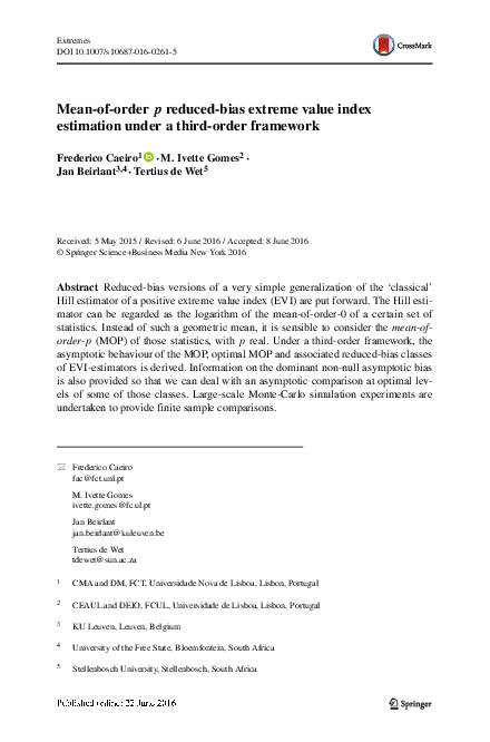
 Tertius de Wet