Pricing weather derivatives in an uncertain environment

Zulfiqar Ali; Javed Hussain; Zarqa Bano

doi:10.1515/nleng-2022-0291

Open Access Published by De Gruyter May 26, 2023

Pricing weather derivatives in an uncertain environment

Zulfiqar Ali , Javed Hussain and Zarqa Bano

From the journal Nonlinear Engineering

https://doi.org/10.1515/nleng-2022-0291

Abstract

This article deals with the problem of finding a pricing formula for weather derivatives based on temperature dynamics through an uncertain differential equation. Weather-related derivatives are being employed more frequently in alternative risk portfolios with multiple asset classes. We first propose an uncertain process that uses data from the past to describe how the temperature has changed. Despite this, pricing these assets is difficult since it necessitates an incomplete market framework. The volatility is described by a truncated Fourier series, and we provide a novel technique for calculating this constant using Monte Carlo simulations. With this approach, the risk is assumed to have a fixed market price.

Keywords: weather derivatives; uncertain temperature; option pricing

1 Introduction

Weather derivatives are financial tools that help organizations and individuals manage the risk associated with unfavorable or unforeseen weather events. Although weather risks affect several industries, such as energy providers and users, grocery chains, agricultural businesses, and the leisure industry, the energy sector has predominantly driven the growth of weather derivatives. These derivatives have underlying variables like rainfall, temperature, humidity, or snowfall and are similar to conventional contingent claims that depend on the price of some fundamental. The market for weather derivatives is growing, and derivatives depending on temperature are the most common. Weather derivatives offer more flexibility than traditional insurance, covering the negative effects of weather on profitability and sales volume, with quantifiable values of the weather used to determine the ultimate settlement payment. Various pricing techniques, including actuarial method, historical burn analysis, and index modeling, have been employed for pricing weather derivatives. However, daily average temperature (DAT) modeling is currently the least computationally demanding method and has been found to be more accurate than the others. Nevertheless, it is challenging to derive a reliable scheme for the daily average temperature.

Weather derivatives have emerged as a more flexible alternative to traditional insurance contracts since they can protect against the negative effects of weather on soft skills, such as profitability and sales volume [1]. Since October 2003, European call-and-put options and conventional futures contracts with temperature indices have been traded on the Chicago Mercantile Exchange (CME) [2]. However, since temperature is the most frequent underlying variable, weather derivatives that depend on temperature necessitate an incomplete market architecture, as the options underlying temperature indices are not traded. Therefore, to fully recognize the risks associated with such trading, comprehensive pricing schemes must be used for both options and futures [3]. Pricing algorithms for temperature-based weather derivatives must take into account the dynamics of daily temperature, which is challenging due to its high localization attribute. As a result, a pricing scheme must be developed for each city where trading is relevant to capture temperature dynamics accurately.

Recently, a great deal of work has been done on the pricing of weather-dependent derivatives. Chuang et al. [4], proposed a generalized model with three components to account for the conditional variance of daily average temperature and derived a closed-form pricing formula for cooling degree day (CDD)/heating degree day (HDD) futures, with empirical results showing asymmetric effects, positive covariance of temperature and variance, and a positive temperature risk premium. Hess [5,6] introduced new temperature and electricity spot price models that capture empirical behavior, with the former based on generalized Langevin equations driven by L é vy processes and the latter explicitly dependent on outdoor temperature, allowing for the derivation of meteorological temperature forecast curves and pricing formulas for diverse electricity and temperature futures contracts, as well as investigations into risk-neutral price dynamics and the minimal variance hedging portfolio in a specific temperature futures market, and the pricing of related derivatives under weather forecasts modeled by an initially enlarged filtration. Cabrales et al. [7] developed a methodology for temperature option pricing in equatorial regions by combining deterministic and stochastic models to forecast daily temperature, calibrated it with data from Bogotá, Colombia, and found the most accurate model to be a truncated third-order Fourier series combined with a mean reversion stochastic process. Bobriková [8] demonstrated that the application of weather derivatives in agriculture can effectively manage weather risk and reduce yield volatility as demonstrated by the evaluation of hedging efficiency against excess rainfall in the crop cycle in the Kosice region of Slovakia using the Burn analysis valuation method. Masala et al. [9] utilized a financial econometrics approach using the spot market price simulation model to derive weather risk exposure in a hypothetical wind farm’s industrial portfolio and demonstrated through a hypothetical hedging strategy with collar options that accurate risk management can lead to substantial benefits in terms of worst-case scenarios. Shibabaw et al. [10] studied a stochastic model with a generalized hyperbolic process to calculate the premium of weather index insurance on temperature indices for three major crops in Ethiopia and calculate the risk factor of the weather derivative market using the growing degree day temperature index, resulting in a more accurate premium value and promising results for establishing weather index insurance. Haung et al. developed a real option model using a power penalty approach to evaluate potential sea level rising risk in Three Gorges Reservoir Area, and a fitted finite volume method is developed to solve the nonlinear parabolic equation in the case of European and American options with an empirical analysis to illustrate theoretical results [11]. Larsson [12] gave a flexible framework for structuring and pricing parametric heat wave insurance based on a general heat wave definition formulated in terms of an underlying temperature index, enabling tailored contracts and using a single stochastic model for pricing all contracts, with an empirical case study performed in Berlin.

Previous option pricing methods were mainly based on Bannor and Scherer [13] pricing option theory, where the price of the underlying asset mechanism is believed to observe stochastic differential equations. On the other hand, in 2009, Liu [14] established European option pricing methods and brought the uncertain differential equation (UDE) into the finance sector, based on the notion that stock prices follow a geometric Liu’s process in uncertainty theory. Moreover, Liu [15] presented a persuasive contradiction to demonstrate that stochastic differential equations are inadequate for describing the stock price mechanism. The practical reality that the underlying asset’s distribution has heavier tails and a greater peak than the typical probability distribution support this viewpoint.

Over the years, the field of uncertain finance has been enriched by numerous research studies that have expanded on the pioneering work of Liu [14]. Specifically, Chen [16] developed formulas for pricing American options by assuming that stock prices follow a geometric Brownian motion process. Sun and Chen [17] provided formulae for pricing Asian options, while Zhang and Liu [18] investigated Asian option pricing formulas using the geometric mean. Gao et al. [19] focused on developing lookback option pricing formulae, and Zhang et al. [20] studied the pricing of exported power options. In addition, Yao [21] presented a no-arbitrage theorem for Liu’s stock. Furthermore, Peng and Yao [22] investigated a mean-reverting uncertain stock model, and Chen et al. [23] proposed an uncertain stock model with periodic dividends. Ji and Zhou [24] introduced an uncertain stock model with jumps, while Yao [25] considered an uncertain stock model with a floating interest rate. Yao’s model assumes that the interest rate and stock price follow two different geometric Liu processes. Dai et al. [26] and Sun et al. [27] developed an uncertain exponential Ornstein-Uhlenbeck (OU) model. In addition, Hassanzadeh and Mehrdoust [28] proposed an uncertain volatility model for European options.

In this study, we aim to develop a pricing formula for weather derivatives by utilizing UDEs to model temperature dynamics. Weather derivatives are becoming more prevalent in alternative risk portfolios that encompass multiple asset classes. To achieve this, we introduce an uncertain process that utilizes historical temperature data to describe its evolution. Nevertheless, pricing these derivatives poses a challenge due to the incomplete market framework. To determine the volatility, we propose a truncated Fourier series, and we offer a unique method for computing this constant using Monte Carlo simulations. Our approach assumes that the risk has a fixed market price. The article is organized as follows.

2 Preliminary

The following is a certain preliminary understanding of uncertainty theory that is required for the formulation and discussion of option pricing problems in an uncertain environment. We assume that Ω be non-empty set and Σ denotes a σ -algebra on Ω .

Definition 2.1

[29] (Uncertain measure) A map ℳ : Σ → R is called uncertain measure if it satisfies following conditions:

ℳ { Ω } = 1 .
ℳ { ∧ } + ℳ { ∧ c } = 1 , for any set ∧ ∈ Σ .
For all ∧ 1 , ∧ 2 ∈ Σ such that ∧ 1 ⊂ ∧ 2 , we have ℳ { ∧ 1 } ≤ ℳ { ∧ 2 } .
For any countable sequence of events { ∧ i } , we have
ℳ ⋃ i = 1 ∞ ∧ i ≤ ∑ i = 1 ∞ ℳ { ∧ i } .
For given uncertainty spaces ( Ω k , Σ k , ℳ k ) k ∈ N , the product uncertain measure ℳ defined on the product σ -algebra ∏ k = 1 ∞ Σ k on ∏ k = 1 ∞ Ω k satisfies
ℳ ⋂ k = 1 ∞ ∧ k = ∏ k = 1 ∞ ℳ { ∧ k }
where ∧ k are arbitrarily chosen events from Σ k .

Definition 2.2

[29] (Uncertain variable) A function X : Ω → R is called uncertain variable for any Borel set B , we have X − 1 ( B ) ∈ Σ .

Definition 2.3

[29] (Uncertain normal distribution) A map Φ : R → [ 0 , 1 ] is called uncertainty distribution of an uncertain normal variable X , if

(2.1) Φ ( v ) = ℳ { X ≤ v } = 1 + exp − π v 3 t − 1 ,

(2.2) 1 − Φ ( v ) = ℳ { X ≥ v } = 1 + exp π v 3 t − 1 ,

for all v ∈ R .

Definition 2.4

[29] (Expectation) For an uncertain variable X , the expected value of X is defined as follows:

E [ X ] = ∫ 0 + ∞ ℳ { X ≥ v } d v − ∫ − ∞ 0 ℳ { X ≤ v } d v .

Definition 2.5

[29] (Variance) For an uncertain variable X , the variance of X can be defined as follows:

Var [ X ] = E [ ( X − E ( X ) ) 2 ] .

Definition 2.6

[29] (LIU’s Process) A time-indexed sequence of uncertain variables C t is called a Liu’s process if:

C 0 = 0
For a ≤ b ≤ c ≤ d , the increments C b − C a and C d − C c are independent in uncertain sense.
For each t ≥ s , the increment uncertain C t + s − C s follows an uncertain normal distribution with parameters mean 0 and variance t 2 :
Φ ( v ) = 1 + exp − π v 3 t − 1 ,
where v is a real number.

Definition 2.7

[29] (UDE) Suppose, C t be Liu’s process, and μ and σ be two functions. Then

(2.3) d S t = f ( t , S t ) d t + g ( t , S t ) d C t ,

is called UDE with initial value S 0 .

The UDE Eq. (2.3) is equivalent to uncertain integral equation,

(2.4) S t = S 0 + ∫ 0 t μ ( t , S t ) d t + ∫ 0 t σ ( t , S t ) d C t ,

where S t is the solution called Liu’s process that satisfies Eq. (2.3).

Example 1

Let μ and σ are two constant functions in differential Eq. (2.3).

(2.5) d S t = μ d t + σ d C t .

It has solution,

(2.6) S t = S 0 + ∫ 0 t μ d t + ∫ 0 t σ d C t ,

which can be written as follows:

(2.7) S t = S 0 + μ t + σ C t .

Theorem 2.1

([14], Product rule) Let X t and Y t be two Liu’s process, then

(2.8) d ( X t Y t ) = Y t d X t + X t d Y t .

Chen and Liu [30] proved the existence and uniqueness theorem for UDEs.

Many writers use mean-reverting OU processes to model temperature dynamics due to the cyclical nature of the data. The temperature model presented is

(2.9) d T t = α ( m t − T t ) d t + σ d C t ,

where C t is the uncertain canonical Liu’s process, a is the rate of mean reversion, m t is the seasonal mean, and σ is the process volatility. To depict the temperature’s mean-reverting dynamics, we need E ( T t ) ≈ m t , but solving Eq. (2.9) leads to T s = m s = C . To fix this issue, Davis [31] suggests including the term d m t d t in the model, resulting in the final model:

(2.10) T t = α ( m t − T t ) + d m t d t d t + σ d C t .

The solution of Eq. (2.10) is

(2.11) T t = m t + e − ∫ s t α d u ∫ s t e ∫ s t α d u σ u d C u .

Research on continuous process uncertain modeling of daily average temperature has primarily focused on the parameter α . The seasonal mean of temperature, represented by m t , is a key factor in the trend of seasonality in the daily average temperature time series. In addition, σ is used to measure volatility. Some studies assume constant volatility and mean reversion speed, while others, like Alaton et al. in [32], assume model volatility as a piece-wise constant function that reflects monthly variations.

2.1 Basic concepts in weather derivatives

To hedge the various risks associated with weather, it is crucial to understand the underlying weather variables that define weather derivatives, as weather affects different entities in different ways. Temperature is the most commonly used weather variable due to its significant impact on financial performance. Temperature values can be expressed as hourly values, daily minimums and maximums, or daily averages, with degree days, average temperature, cumulative average temperature, and event indices being the most commonly used temperature indices for weather derivative contracts. By using these indices, one can hedge against potential financial losses due to deviations in weather patterns, particularly for industries such as agriculture, energy, and tourism that are directly affected by weather.

Definition 2.8

[32] A degree day represents the variance between a standard temperature and the mean temperature observed on a particular day.

The daily average temperature T i for day i is defined as follows:

T i = T i max + T i min 2 .

Here, T i max and T i min represent the maximum and minimum temperatures, respectively, observed on day i [1]. In most literature on weather derivatives, the base temperature is defined as the temperature level that triggers the activation or deactivation of heating or cooling systems. We denote this base temperature by T base , which is conventionally set to 18°C (or 65°F) [1]. This is because weather conditions can exceed T base during the summer and fall below it during the winter. However, temperature movements are not symmetric around the base temperature T base . In some cases, although rare, temperatures may fall below T base during the summer, or may exceed or not reach it during the winter. There are two types of temperature indices used for degree days: HDDs and CDDs.

Definition 2.9

[32] HDD indices are used to measure the coldness of a day and provide information on the number of degrees by which the daily average temperature T i falls below the base temperature T base . This is expressed by the following equation:

HDD i = max { 0 , T base − T i } .

The HDD index, HDDs, for a contract period spanning m days is calculated as the sum of HDDs over all days:

HDDs = ∑ t = 1 m HDD i .

Definition 2.10

CDD indices measure how hot the day was. It tells us how many degrees of temperature the daily average temperature T i was above the base temperature T base . It is given as follows:

CDD i = max { 0 , T i − T base } .

Then, the CDDs index, CDDs over N days period is the sum of CDDs over all days during the contract period, i.e.,

CDDs = ∑ t = 1 m CDD i

The usage of degree day indices in the weather market is quite popular. These indices are used to measure the amount of energy used by customers in their heating systems or air conditioners. HDDs and CDDs are the two most popular degree day indices. CDDs are of most relevance to participants in the gas market because more electricity is now generated from natural gas. There is a high correlation between HDDs and power and gas use in the United States, and the consumption of gas is highly correlated with temperature variations. The CME offers options and futures contracts based on the HDD and CDD indices, which represent daily accumulations of HDD and CDD during a specific season or month.

A call option protects an investor from high index levels, while a put option protects a firm from low index levels. When creating a general weather option, various parameters such as the type of contract, period, underlying index, temperature data, strike threshold, tick size, and highest possible payoff should be considered. The formula for determining an option’s payoff involves using γ and K to represent the tick size and strike level, respectively. The contract period is m days, and the number of HDDs and CDDs for that time period is calculated using

(2.12) H m = ∑ i = 1 m HDD i and C m = ∑ i = 1 m CDD i ,

respectively. The payoff of an uncapped HDD call may now be written as follows:

(2.13) f c = γ max { H m − K , 0 } .

Payouts for related contracts such as HDD puts and CDD calls/puts are specified similarly.

3 Modeling temperature

In this section, we aim to find a continuous uncertain process that can accurately describe temperature changes. Our method aligns with the principles outlined in ref. [32]. We utilized temperature data from several Swedish cities over the past 40 years to identify a suitable model. Figure 1 illustrates the average daily temperatures at Stockholm Bromma Airport over a 9-year period, demonstrating a cyclical pattern and oscillation around a seasonal mean influenced by urbanization trends. Following ref. [33], we propose using a mean-reverting OU process to model the dynamics of daily average temperatures. As a result, in keeping with [31], we use the mean reverting OU process to describe the dynamics of DAT:

(3.1) d T t = d g ( t ) d t + α ( g ( t ) − T t ) d t + σ t d C t .

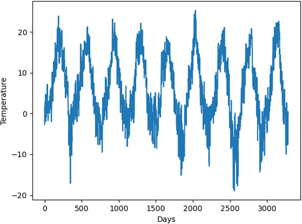
We use the linear technique from [1] to determine the functional form of S ( t ) and σ ( t ) and estimate the value of the constant α .

Figure 1

Daily average temperature at Bromma Airport during 1990–1999.

3.1 Modeling non-random seasonal average and trends of temperature

Figure 1 displays a temperature time series with consistent peaks and a mild rising trend. Alexandridis and Zapranis [2] proposes that the temperature trend can be modeled with a linear function, and the seasonality can be represented using a single sine function. Thus, the predictable seasonal temperature can be modeled using the following equation:

(3.2) g ( t ) = A 1 + A 2 t + A 3 sin ( ω t + ϕ ) ,

where ω = 2 π 365 is the duration, and ϕ is the phase shift that captures the maximum and minimum temperatures. However, using a general periodic function such as (3.2) would suggest that the annual minimum and maximum temperatures occur on the same day of the year and have constant values, which are not accurate.

To obtain accurate parameter values for Eq. (3.2), the method of least squares was used, which involves estimating the values of the parameters using historical data. By minimizing the estimate errors, Eq. (3.2) can be represented in the following form:

(3.3) g ( t ) = c 1 + c 2 t + c 3 sin ( ω t ) + c 4 cos ( ω t ) .

Using numerical values in Eq. (3.2), the following relation was obtained for the average temperature:

(3.4) g ( t ) = 5.96 + 6.56.1 0 − 5 t + 10.4 sin 2 π 365 t − 2.01 .

Furthermore, it was observed that the weak linear trend in the temperature time series is highlighted by the extremely low coefficients of t in the equations.

To determine the mean reversion speed, we use a linear approach. First, note that by employing the Euler discretization scheme, the UDE (3.1) can be changed into:

(3.5) T t − T t − 1 = T t n − T t − 1 n + α ( T t n − T t ) d t + σ t ζ ( t ) ,

where ζ ( t ) is standard uncertain normal variable. Using the transformation T ¯ t = T t − T t n , we obtain the following (which is the same as detrending and deseasonalizing the DAT):

(3.6) T ¯ t = β T ¯ t − 1 + e ( t ) ,

where α = 1 − β and e ( t ) = σ t ζ ( t ) . Using the historic data in Eq. (3.6), we obtain α = 0.237 .

3.2 Modeling standard deviation of temperature

In this section, we determine the true value of σ from the data, deviating from the approach in ref. [32] and instead following the methods outlined in refs [2] and [34]. These articles model temperature volatility using Fourier series. We take a similar approach for volatility,

σ ( t ) = q + ∑ n = 1 N C n sin ( n ω t ) + ∑ m = 1 M d m cos ( m ω t ) .

To represent the trend in the annual volatility, we substitute a linear component for the constant q , i.e., the fact that winter months see more volatility than summer months. As a result, the volatility is determined as follows:

σ ( t ) = X + Y t + ∑ n = 1 N C n sin ( n ω t ) + ∑ m = 1 M d m cos ( m ω t ) .

Reasonable values for N , M , and the related constants are determined using historical data. After determining the average variance for the 24 h of data for each day of the year, the best model for these values is then obtained using the least squares method.

4 Winter valuation of HDD and CDD contracts

We assume that temperature on a typical day follows UDE driven by Liu’s process ( C t ) t ≥ 0 :

(4.1) d T t = d g ( t ) d t + α ( g ( t ) − T t ) d t + σ t d C t .

In order to explicitly solve this UDE we aim to apply the formula from Chen and Ralescu [35],

d h ( t , x ) = d h d t + μ d h d x d t + σ d h d x d C t ,

to the following function:

(4.2) h ( t , x ) = exp ( α t ) ( x − g ( t ) ) ,

where the coefficients μ and σ are the drift and diffusion. By integrating both sides from s to t , we obtain:

(4.3) T t = g ( t ) + ( T s − g ( s ) ) exp ( − α ( t − s ) ) + σ t ∫ s t exp ( α ( t − u ) ) d C u ,

and the above equation provides us

(4.4) Var [ T t ] = σ t ∫ s t exp ( α ( t − u ) ) d u

and

(4.5) E [ T t ] = g ( t ) + ( T s − g ( s ) ) exp ( − α ( t − s ) ) .

This study focuses on temperature-based weather derivatives. The temperature is modeled uncertainly and is a good estimation of the original data. Studies have shown that weather derivatives can be priced based on degree days for heating or cooling. The formula for HDD call and put options is given, with the payout for the HDD call option being

f c = ( H m − K ) + ,

where H m is calculated as the sum of the maximum temperatures that are below 18°. The payout is similar to an Asian option, but the maximum temperature creates complications for finding an explicit solution. For winter, the maximum temperature is usually zero, making it simple to find an explicit solution. The payout can be written as follows:

f c = 18 m − ∑ m = 1 M T t i − K + ,

which is normally distributed because the temperature is normally distributed.

The price of a call option on a winter weather derivative at any time s ≤ t comes from the fundamental theorem of asset pricing,

C ( t ) = e − r ( t − s ) E [ ( H m − K ) + ] , = e − r ( t − s ) ∫ 0 ∞ ℳ ( H m − K ≥ s ) d s , = e − r ( t − s ) ∫ 0 ∞ ℳ 18 m − ∑ m = 1 M T t i − K ≥ s d s , = e − r ( t − s ) ∫ 0 ∞ ℳ 18 m − ( g ( t ) + ( T s − g ( s ) ) e − α ( t − s ) + λ α σ t ( 1 − e − α ( t − s ) ) + σ t ∫ s t e − α ( t − s ) d C u ) − K ≥ s d s , = e − r ( t − s ) ∫ δ ∞ ℳ e − r ( t − s ) ∫ s t − σ t e − α ( t − s ) d C u ≥ s d s ,

where

δ = K − 18 m + g ( t ) + ( T s − g ( s ) ) e − α ( t − s ) + λ α σ t ( 1 − e − α ( t − s ) ) .

Since ∫ s t − σ t e − α ( t − s ) d C u ∼ N ( 0 , ∫ s t ∣ − σ t e − α ( t − s ) ∣ d u ) (in uncertain sense), it follows that

C ( t ) = e − r ( t − s ) ∫ δ ∞ ℳ σ t α ( 1 − e − α ( t − s ) ) ζ ≥ s d s ,

where ζ is standard normal uncertain variable. The above equation can be further simplified as follows:

(4.6) C ( t ) = e − r ( t − s ) ∫ δ ∞ ℳ ζ ≥ α s σ t ( 1 − e − α ( t − s ) ) d s , = e − r ( t − s ) σ t α ( 1 − e − α ( t − s ) ) ∫ β ∞ ℳ ( ζ ≥ s ) d s , = e − r ( t − s ) σ t α ( 1 − e − α ( t − s ) ) ∫ β ∞ 1 + e − π s 3 t − 1 d s , C ( t ) = 3 π t e − r ( t − s ) σ t α ( 1 − e − a ( t − s ) ) ln 1 + e − π β 3 t ,

where β = α δ σ t ( 1 − e − α ( t − s ) ) . Eq. (4.6) gives the pricing formula for the HDD call option.

Using the identical contract details as a put option and the aforementioned transformations, the price of a put option is then calculated as follows:

P ( t ) = e − r ( t − s ) E [ ( K − H m ) + ] = e − r ( t − s ) ∫ 0 ∞ ℳ ( K − H m ≥ s ) d s , = e − r ( t − s ) ∫ 0 K ℳ K − 18 m + ∑ m = 1 M T t i ≥ s d s , = e − r ( t − s ) ∫ 0 K ℳ K − 18 m + g ( t ) + ( T s − g ( s ) ) e − α ( t − s ) + λ σ t α ( 1 − e − α ( t − s ) + σ t ∫ s t e − α ( t − s ) d C u ) − K ≥ s d s , = e − r ( t − s ) ∫ − δ K − δ ℳ e − r ( t − s ) ∫ s t σ t e − α ( t − s ) d C u ≥ s d s , = e − r ( t − s ) ∫ − δ K − δ ℳ σ t α ( 1 − e − α ( t − s ) ) ζ ≥ s d s , = e − r ( t − s ) ∫ − δ K − δ ℳ ζ ≥ α s σ t ( 1 − e − α ( t − s ) ) d s , = σ t α e − r ( t − s ) ( 1 − e − α ( t − s ) ) ∫ γ β ℳ ( ζ ≥ s ) d s , = σ t α e − r ( t − s ) ( 1 − e − α ( t − s ) ) ∫ γ β 1 + e − π s 3 t − 1 d s , P ( t ) = 3 π σ t a t e − r ( t − s ) ( 1 − e − α ( t − s ) ) ln 1 + e − π β 3 t − ln 1 + e − π γ 3 t ,

where

δ = K − 18 m + g ( t ) + ( T s − g ( s ) ) e − α ( t − s ) + λ α σ t ( 1 − e − α ( t − s ) ) , γ = − δ α σ t ( 1 − e − α ( t − s ) ) , β = ( K − δ ) α σ t ( 1 − e − α ( t − s ) ) .

5 Numerical simulations and interpretations

5.1 Monte Carlo simulations

In this section, we will not make any assumptions about the distribution of H m or any other variable. Instead, we will use the Monte Carlo simulation method to calculate the expected value E [ f ( Y ( t ) ) ] , where Y is the solution to a UDE and f is a function. This is done by simulating multiple process trajectories and taking the arithmetic mean of the results to estimate the projected outcome. The equation used for this estimation is

E [ f ( Y ( t ) ) ] ≈ 1 K ∑ n = 1 K f ( Y ¯ ( t , b i ) ) ,

where Y ¯ is an approximation of Y and must be used when the exact solution Y is not available.

When simulating temperature paths over a certain time period, we have two options: we can either begin the simulation immediately with the current temperature as the initial value, or, if the contract period is far enough in the future, we can start the simulation on a future date, using the predicted average temperature for that day as the initial value. The reason for this is that if the contract period is far enough in the future, the forecasted temperature will not have a significant impact on the temperature during the contract period, as the variance will eventually reach a stable state and the temperature process will no longer be dependent on the initial value. However, if the contract period is relatively close or has already begun, it is more appropriate to begin the simulations at the present time.

5.2 Estimating the market price of risk

As discussed in the previous section, we should model temperature trajectories by simulating the dynamics of temperature from Eq. (3.1). To do this, we must first determine estimates for the parameter λ , which describes the risk preferences of weather traders. This can be done by analyzing market pricing for weather derivative contracts and selecting the best value of λ for which our model produces prices that are comparable to these. As the market for weather derivatives is still relatively new, there may not be many contracts available to support this strategy. Therefore, it is suggested that the best estimate for the value of λ is when the predicted degree days are close to the observed degree days.

To estimate the value of λ , we use test data and run Monte Carlo simulations. Specifically, we conducted 20,000 Monte Carlo simulations of temperature trajectories for the month of January, using the values predicted in [7] as a reference:

λ ∈ { − 1.0 , … − 0.01 , 0.0 , 0.01 , … 1.0 } .

6 Results

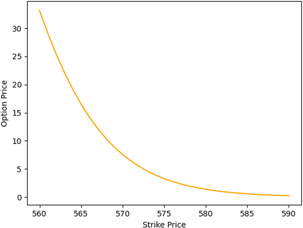
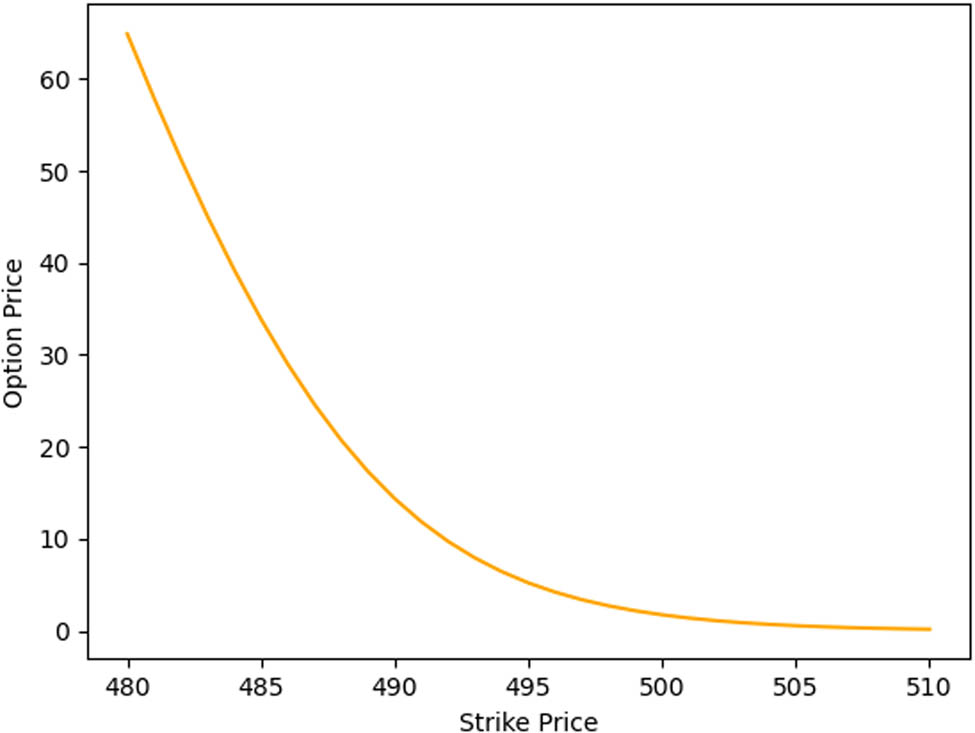
In this section, we will compare the costs of several contracts using both an approximation formula and the Monte Carlo simulation method. To estimate the costs, we used the Monte Carlo simulation technique with 20,000 sample paths. Using the model proposed in this work, we calculated the price of a call option with index HDD for the months of January, February, and March at Bromma Airport Stockholm, with strike levels of 525 HDD s , 650 HDD s , and 480 HDD s , respectively (Table 1 and Figures 2 and 3).

Table 1

The prices of the different options

Formula	Option I	Option II	Option III
Uncertain formula	55.6	33.1	64.8
Approximation formula	55.7	33.0	64.4
Monte Carlo	56	33.3	65

Figure 2

February.

Figure 3

March.

7 Conclusion

In recent years, weather derivatives have gained popularity on the CME, attracting interest from both hedgers and investors. These options are appealing to investors because they offer a robust defense against daily weather uncertainty and have a low correlation with other market factors. However, one of the main challenges in pricing and trading these derivatives is the nature of the underlying.

In this study, we aimed to find pricing formulas for weather derivatives at Swedish Bromma Airport. Our objective was to identify closed-form pricing formulas for call and put options based on HDD/CDD indices as well as continuous uncertain processes for determining temperature progression. We presented the use of Monte Carlo simulations to determine these constants under the assumption that risk has a fixed market price. This study provides a more practical and beneficial approach when looking at the objective functions created by the firm itself. The model offers a customized price depending on temperature risk in order to meet a target in terms of profit.

Funding information: The authors did not receive any external funding to perform this research.
Author contributions: All authors have accepted responsibility for the entire content of this manuscript and approved its submission.
Conflict of interest: The authors declare that they have no conflict of interest.
Data availability statement: No data were required to perform this research.

References

[1] Jewson S. Introduction to weather derivative pricing. J Altern Invest. 2004;7:57–64. 10.3905/jai.2004.439646Search in Google Scholar

[2] Alexandridis A, Zapranis AD. Weather derivatives: modeling and pricing weather-related risk. New York (NY), USA: Springer Science & Business Media; 2012. 10.1007/978-1-4614-6071-8Search in Google Scholar

[3] Benth FE, Saltyte-Benth J. Stochastic modelling of temperature variations with a view towards weather derivatives. Appl Math Finance. 2005;12(1):53–85. 10.1080/1350486042000271638Search in Google Scholar

[4] Chuang MC, Shih PT, Li SW, Lin SK. A closed-form solution for Cdd/Hdd futures under the generalized model: an empirical application. SSRN. February 25, 2022. https://ssrn.com/abstract=4043651 or 10.2139/ssrn.4043651. Search in Google Scholar

[5] Hess M. Pricing and hedging of temperature derivatives in a model with memory. SSRN. December 21, 2022. https://ssrn.com/abstract=4308980 or 10.2139/ssrn.4308980. Search in Google Scholar

[6] Hess M. Modeling the impact of temperature variations on electricity prices. SSRN. February 17, 2023. https://ssrn.com/abstract=4362636 or 10.2139/ssrn.4362636. Search in Google Scholar

[7] Cabrales S, Bautista R, Madiedo I, Galindo M. A methodology for temperature option pricing in the equatorial regions. Eng Economist. 2022;60(2):96–11110.1080/0013791X.2021.2000086Search in Google Scholar

[8] Bobriková M. Weather risk management in agriculture using weather derivatives. Italian Rev Agric Econ. 2022; 77(2):15–26. 10.36253/rea-13416. Search in Google Scholar

[9] Masala G, Micocci M, Rizk A. Hedging wind power risk exposure through weather derivatives. Energies. 2022;15(4):1343. 10.3390/en15041343. Search in Google Scholar

[10] Shibabaw A, Berhane T, Awgichew G, Walelgn A, Muhamed AA. Hedging the effect of climate change on crop yields by pricing weather index insurance based on temperature. Earth Syst Environ. 2023;7:211–21. 10.1007/s41748-022-00298-x. Search in Google Scholar

[11] Huang F, Lu Z, Li L, Wu X, Liu S, Yang Y. Numerical simulation for European and American option of risks in climate change of three gorges reservoir area. J Numer Math. 2022;30(1):23–42. 10.1515/jnma-2020-0081. Search in Google Scholar

[12] Larsson K. Parametric heat wave insurance. SSRN. November 4, 2022. https://ssrn.com/abstract=4268564 or 10.2139/ssrn.4268564. Search in Google Scholar

[13] Bannor KF, Scherer M. Model risk and uncertainty-illustrated with examples from mathematical finance. In: Klüppelberg C, Straub D, Welpe IM, editors. Risk-A multidisciplinary introduction. Cham, Switzerland: Springer; 2014. p. 279–306. 10.1007/978-3-319-04486-6_10Search in Google Scholar

[14] Liu B. Some research problems in uncertainty theory. J Uncertain Syst. 2009;3(1):3–10. Search in Google Scholar

[15] Liu B. Toward uncertain finance theory. J Uncertain Anal Appl. 2013;1(1):1–15. 10.1186/2195-5468-1-1Search in Google Scholar

[16] Chen X. American option pricing formula for uncertain financial market. Int J Operat Res. 2011;8(2):32–7. Search in Google Scholar

[17] Sun J, Chen X. Asian option pricing formula for uncertain financial market. J Uncertain Anal Appl. 2015;3(1):1–11. 10.1186/s40467-015-0035-7Search in Google Scholar

[18] Zhang ZQ, Liu WQ. Geometric average Asian option pricing for uncertain financial market. J Uncertain Syst. 2014;8(4):317–20. Search in Google Scholar

[19] Gao Y, Yang X, Fu Z. Lookback option pricing problem of uncertain exponential Ornstein-Uhlenbeck model. Soft Comput. 2018;22(17):5647–54. 10.1007/s00500-017-2558-ySearch in Google Scholar

[20] Zhang Z, Liu W, Sheng Y. Valuation of power option for uncertain financial market. Appl Math Comput. 2016;286:257–64. 10.1016/j.amc.2016.04.032Search in Google Scholar

[21] Yao K. A no-arbitrage theorem for uncertain stock model. Fuzzy Optim Decision Making. 2015;14(2):227–42. 10.1007/s10700-014-9198-9Search in Google Scholar

[22] Peng J, Yao K. A new option pricing model for stocks in uncertainty markets. Int J Operat Res. 2011;8(2):18–26. Search in Google Scholar

[23] Chen X, Liu Y, Ralescu DA. Uncertain stock model with periodic dividends. Fuzzy Optim Decis Mak. 2013;12(1):111–23. 10.1007/s10700-012-9141-xSearch in Google Scholar

[24] Ji X, Zhou J. Option pricing for an uncertain stock model with jumps. Soft Comput. 2015;19(11):3323–9. 10.1007/s00500-015-1635-3Search in Google Scholar

[25] Yao K. Uncertain contour process and its application in stock model with floating interest rate. Fuzzy Optim Decis Mak. 2015;14(4):399–424. 10.1007/s10700-015-9211-ySearch in Google Scholar

[26] Dai L, Fu Z, Huang Z. Option pricing formulas for uncertain financial market based on the exponential Ornstein-Uhlenbeck model. J Intell Manuf. 2017;28(3):597–604. 10.1007/s10845-014-1017-1Search in Google Scholar

[27] Sun Y, Yao K, Fu Z. Interest rate model in uncertain environment based on exponential Ornstein-Uhlenbeck equation. Soft Comput. 2018;22(2):465–75. 10.1007/s00500-016-2337-1Search in Google Scholar

[28] Hassanzadeh S, Mehrdoust F. Valuation of European option under uncertain volatility model. Soft Comput. 2018;22(12):4153–63. 10.1007/s00500-017-2633-4Search in Google Scholar

[29] Liu B. Uncertainty theory: A branch of mathematics for modeling human uncertainty. Berlin Heidelberg, Germany: Springer; 2010. Search in Google Scholar

[30] Chen X, Liu B. Existence and uniqueness theorem for uncertain differential equations. Fuzzy Optim Decis Mak. 2010;9(1):69–81. 10.1007/s10700-010-9073-2Search in Google Scholar

[31] Davis M. Pricing weather derivatives by marginal value. Quant Financ. 2001;1(3):305–8. 10.1080/713665730Search in Google Scholar

[32] Alaton P, Djehiche B, Stillberger D. On modelling and pricing weather derivatives. Appl Math Finance. 2002;9(1):1–20. 10.1080/13504860210132897Search in Google Scholar

[33] Dornier F, Queruel M. Caution to the wind. Energy Power Risk Manage. 2000;13(8):30–2. Search in Google Scholar

[34] Benth FE, Benth J. The volatility of temperature and pricing of weather derivatives. Quant Financ. 2007;7(5):553–61. 10.1080/14697680601155334Search in Google Scholar

[35] Chen X, Ralescu DA. Liu process and uncertain calculus. J Uncertain Anal Appl. 2013;1(1):1–12. 10.1186/2195-5468-1-3Search in Google Scholar

Received: 2023-02-18

Revised: 2023-04-04

Accepted: 2023-04-13

Published Online: 2023-05-26

This work is licensed under the Creative Commons Attribution 4.0 International License.

Pricing weather derivatives in an uncertain environment

Abstract

1 Introduction

2 Preliminary

Definition 2.1

Definition 2.2

Definition 2.3

Definition 2.4

Definition 2.5

Definition 2.6

Definition 2.7

Example 1

Theorem 2.1

2.1 Basic concepts in weather derivatives

Definition 2.8

Definition 2.9

Definition 2.10

3 Modeling temperature

3.1 Modeling non-random seasonal average and trends of temperature

3.2 Modeling standard deviation of temperature

4 Winter valuation of HDD and CDD contracts

5 Numerical simulations and interpretations

5.1 Monte Carlo simulations

5.2 Estimating the market price of risk

6 Results

7 Conclusion

References

Journal and Issue

Articles in the same Issue