A novel hybrid ensemble convolutional neural network for face recognition by optimizing hyperparameters

2.1 Datasets used

The authors used two standard datasets, namely LFW and CPLFW, and one small self-created criminal dataset to evaluate SOTA for face detection and recognition. Images of different classes of each dataset are shown in Figure 2.

Figure 2

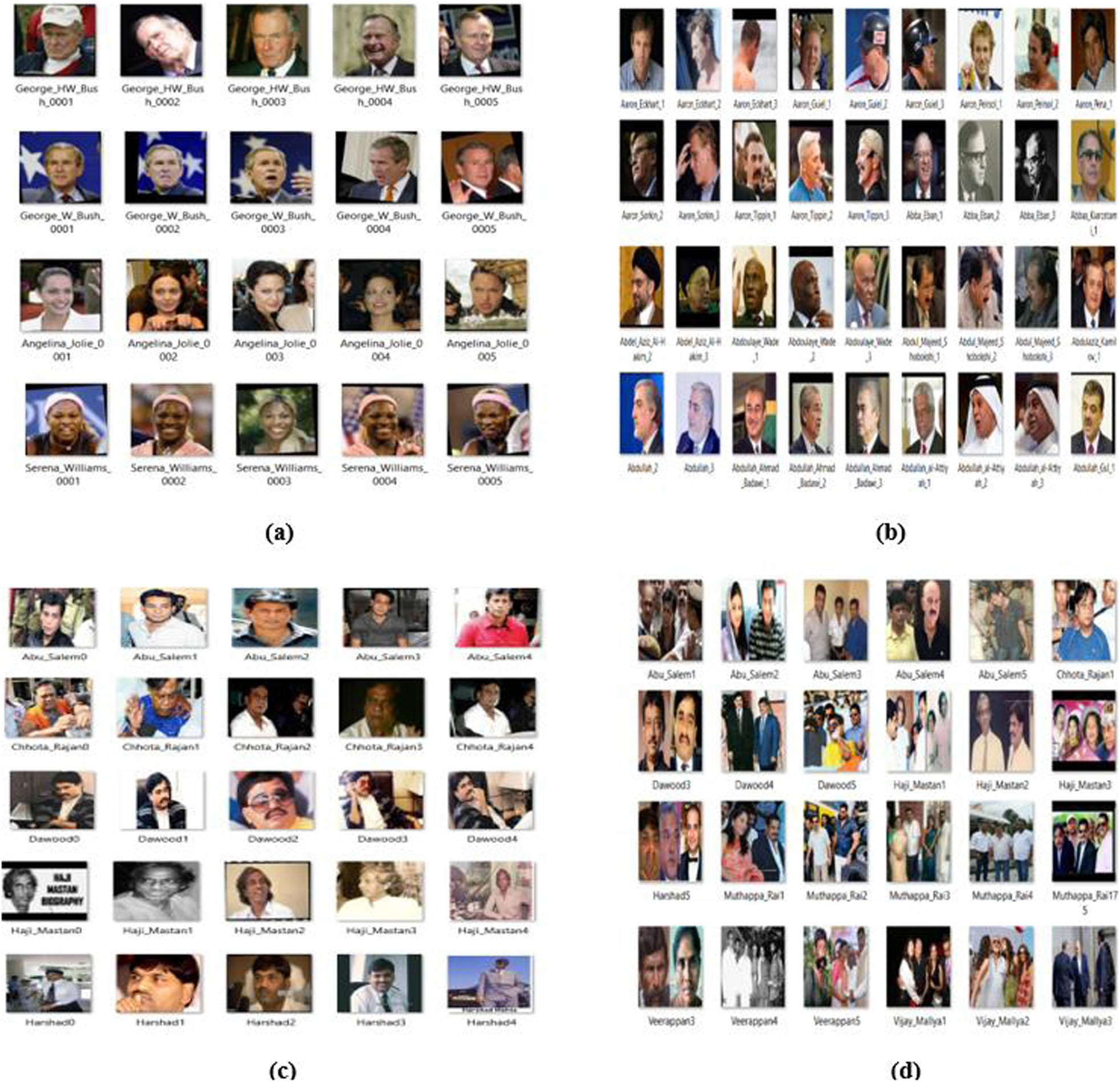
Images of each class of used datasets: (a) LFW, (b) CPLFW, (c) training set of the proposed criminal dataset, and (d) testing set of the proposed criminal dataset.

LFW is a benchmark for face recognition/verification and a publicly available dataset. It was published in 2007 and contained 13,233 images of 5,749 different identities. A total of 1,680 classes having more than one image in the dataset, and 4,096 have only one image in the database. The size of all the images in the dataset is 250 × 250 with a resolution of 96 DPI (dots per inch), and the image format is JPEG. Most faces are frontal and only consider unconstrained factors such as illumination variation and partial occlusion.

CPLFW is the enhanced version of the LFW standard dataset, considering images with significant pose variations. It was published in 2018 and consisted of 11,652 images of 3,928 individuals containing 2 or 3 images of each class. The accuracy of SOTA for face recognition drops by 15–20% on CPLFW compared to LFW, as it contains images with a considerable variation of unconstrained factors.

The main objective of creating the self-created criminal dataset is the class imbalance in LFW. The largest class contains 500 times more images than those in the lowest class. Due to this drawback, the model could bias toward the class having more images (i.e., the class having more images of the same person could recognize the person accurately, but the class having fewer images of the person could lead to a lower recognition rate). In LFW, unconstrained factors like large pose variation and low-resolution images are not considered. The other reason for preparing the criminal dataset is to consider the low-resolution images, as the images in standard datasets like LFW and CPLFW are captured with high-resolution cameras. There are 10 classes in the proposed dataset labeled with the name of the criminal, and all the classes contain 25 images for training the model to ensure the balance of images in each category. Images of the self-created dataset are taken from the internet, and each image’s size is set to 224 × 224 by taking the average height and width of all images. This dataset is designed to present a real-time face recognition application in video surveillance. The surveillance cameras capture images containing multiple people in a single frame to recognize individuals. Therefore, a set of another 50 images is created for testing the proposed model to recognize many faces at once. These 50 images contain the faces of the 10 criminals and other unknown individuals.

2.2 Proposed modified architecture of baseline models

The early layers of the CNN model extract the features, and the last layers are used for the classification. The architectures of the last layers of the used pre-trained models (VGG, ResNet, DenseNet) are delineated in Figure 3.

Figure 3

The architecture of classification layers of pre-trained models (ResNet50, DenseNet169, VGG16, and VGG19).

In this article, the modified architecture of the base models is proposed by adding global pooling, BN, and dropout in the classification layers of models. The pooling layer helps to abbreviate a large number of trainable parameters from the model. Generally, two types of pooling techniques are used, i.e., average and max pooling, which can be mathematically described using the following equations:

where F is the input feature map received from the previous Conv layer, O max n , n ( F ) is the maximum pooling operation on the input feature map of size n × n , O avg n , n ( F ) is the average pooling operation, and P is the output of the pooling layer. It is ascertained that sometimes the maximum value of the activation map n H × n w × n C (where n H is the height, n w is the width, and n C is the channel count in the feature map) received from the last layers gives better performance than the average value and conversely also true. In order to retain both the maximum and average values, we concatenated the max and average values using concatenate function in Keras (https://keras.io). Global pooling helps to reduce each channel in a feature map to a single value and can be used as a substitute for densely connected or FC layers in a classifier. BN effectively normalizes the positive and negative features received from the previous convolutional layer of the model, which helps to reduce the problem of covariate shift [24] and improves accuracy without any side effects [35]. Since we experienced overfitting while training, dropout layers are added for regularization. Dropout is the regularization technique to reduce overfitting. As given in the study of Garbin et al. [35], the dropout value can significantly change the model’s accuracy. Therefore, different values are considered, and we experimentally acquired the optimal dropout value for the model. The non-linearity functions, such as ReLU [36], PReLU [37], leaky ReLU [38], etc., can be placed before or after the BN layer. In our proposal, the use of leaky ReLU after the BN layer gives better results. Therefore, we used the leaky ReLU activation function because it alleviates the problem of “dying ReLU” [38]. The mathematical expression for calculating the value of leaky ReLU is given in the following equation:

The function produces a value of x when the given input is positive, but if the input is negative, it will output a minimum value of 0.01 × x . Therefore, leaky ReLU gives the output for the negative input also. This modification in ReLU leads to a non-zero gradient at the left side of the mathematical graph. In this way, dead neurons will be removed from that region. The modified architecture of the baseline model is shown in Figure 4. The persuasive reasons for the modification in the architecture of baseline models are discussed in Table 1.

Figure 4

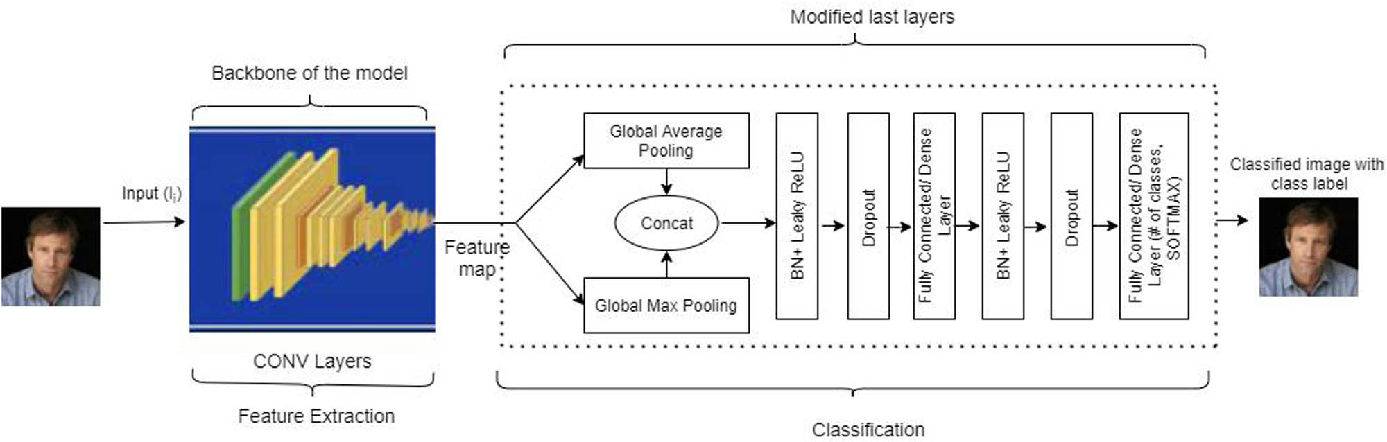
The modified architecture of the baseline model consisting of gmp, gap, BN, dropout, and FC layers (the dotted line shows the modified part of the model).

2.3 Model training and hyperparameter tuning

In the proposed approach, model training is done in the following two steps.

Step 1: First, freeze the early layers in the network and train only classification layers. However, the initial layers (i.e., the feature extraction layers) are not trained during the first step of training the network.

Step 2: Then, a fine-tuned model is loaded from step 1, and all the layers are unfreezed to train the complete model. Figure 5 provides a visual representation of the entire procedure.

Figure 5

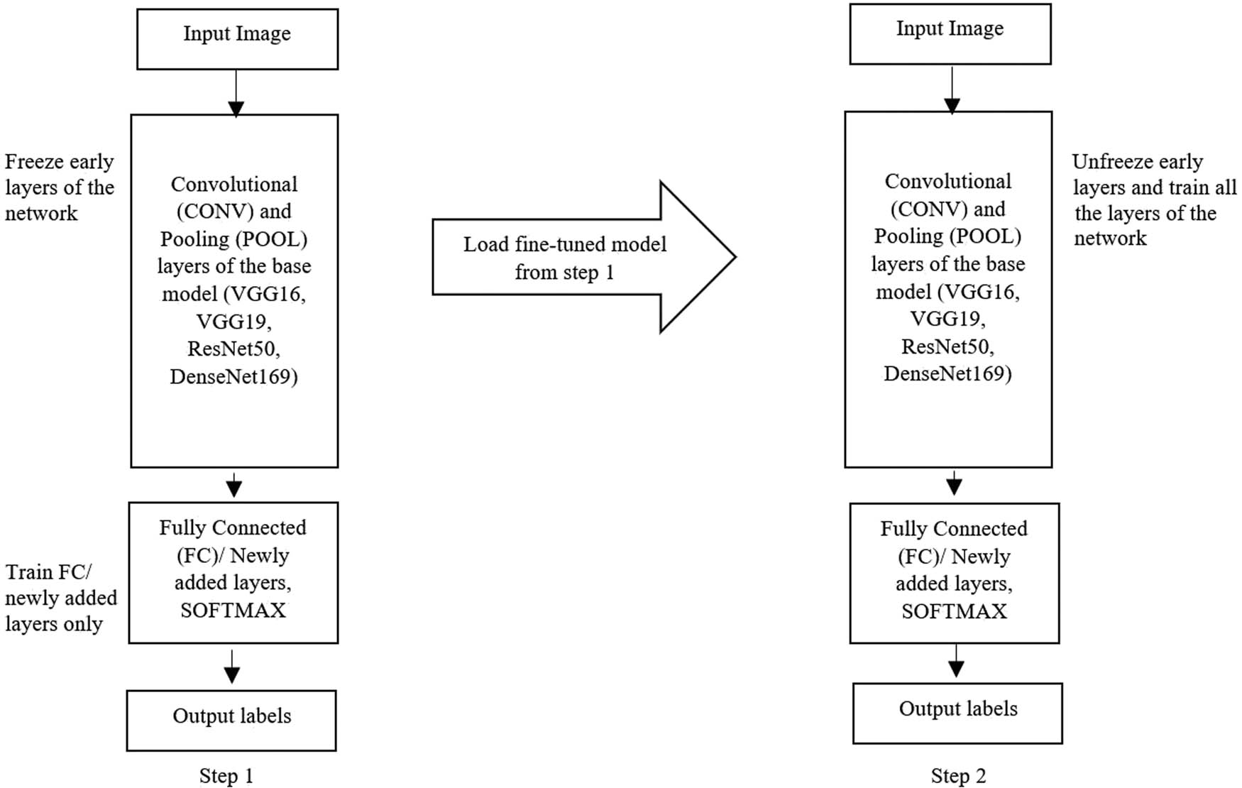
Steps for training the models.

The model’s training process involves implementing a one-cycle policy [39], which replaces the fixed learning rate with cyclical learning rates. Hyperparameter tuning has proven to be an effective solution to improve machine learning model accuracy. In the conferred approach, tweaking of the learning rate, batch size, image size, epoch, and drop-out is done experimentally in Section 3.2 to tune the pre-trained models for the addressed task. The selection of learning rate should be chosen wisely; if it is too large, the optimal value may be an overshoot, and if it is too small, it will require too many iterations to converge to the best value. Therefore, the learning rate finder (LRF) curve [39] is used to locate the optimal learning rate for the model. The LRF is a valuable tool for automatically determining a reasonable learning rate for any model. For example, the red dot in Figure 6 illustrates the optimal learning rate for the deep learning model. The learning rate is gradually raised from an exponentially low value (e.g., 10⁻⁶) to a high value (e.g., 1) while training the data in small batches. During the cool-down phase, the training rate oscillates between a lower and higher learning rate boundary before returning to its initial low boundary. A one-hot vector is created through conversion to predict the class of data while employing categorical cross-entropy as the loss function in Eq. (4) within the softmax layer:

where n is the count of images in training data, i is the index of the input image (i.e., ith image), j is the class’s index, y ij is the one-hot encoded label, and p ij is the probability distribution over C classes. Adam [40] optimizer is used for the optimization of the model.

Figure 6

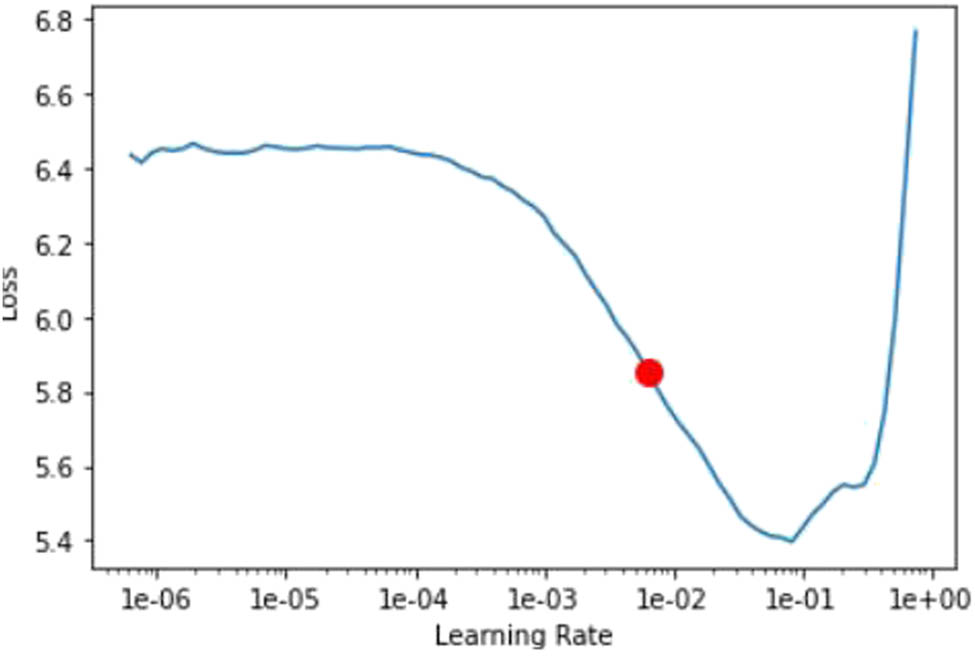
The LRF curve.

2.4 Proposed HE-CNN framework

Algorithm 1 acquires the optimized baseline models and utilizes the ensemble learning approach to get an efficacious hybrid model. Ensemble learning combines the predictions of more than one model to produce the optimal predictive model for the addressed task. The stacking approach of ensemble learning is used to design a hybrid model for the face recognition problem. The final prediction of the hybrid model is made by aggregating the results obtained from the fine-tuned baseline models by conducting a weighted sum operation. The weighted sum or weighted average [41] operation is often applied to ensemble models to give more importance to the predictions of the better-performing models. The idea behind the weighted sum operation is to assign different weights to the predictions of each model in the ensemble based on their relative performance on a validation set. The better-performing models are given higher weights, while the poorer-performing models are assigned lower weights. This means that the final prediction of the ensemble will be more influenced by the predictions of the better models and less influenced by the predictions of the poorer models. Using a weighted sum operation on ensemble models, we can leverage the strengths of multiple models and minimize their weaknesses. This can lead to better overall performance and more robust predictions [42]. The predicted face using the hybrid ensemble model ( P HE − CNN ) is defined in Eq. (5). VGG19 shows better accuracy in Tables 3 and 5. As a result, the VGG19 version is chosen above the VGG16 variant. However, we considered VGG19, DenseNet169, and ResNet50 in the hybrid model. The complete procedure is shown in Figure 7:

where W i denotes the weight of rectified baseline models, § = 3 because we considered three models for the ensemble framework, n is the count of image samples in training data, C is the number of classes in a dataset, f ( j ) is the feature of the j th sample, θ is the parameter matrix of the softmax loss function L ( θ ) , and θ k T f ( j ) is the inner product of θ k and f ( j ) . The optimal values of W 1 , W 2 , and W 3 are selected using VotingClassifier available in the scikit-learn library of Python (https://rb.gy/p0ig).

Figure 7

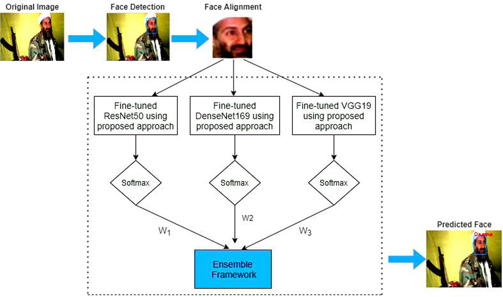
The proposed HE-CNN framework.

Algorithm 1: Algorithm of the proposed approach for training to obtain fine-tuned models

Input: Training Dataset D = { x i , y i } i = 1 n , where n is the count of input images in the dataset

   Pre-trained CNN model (here, VGG16, VGG19, ResNet50 and DenseNet169 are taken)

   No. of epochs (e)

   Batch size (α)

   Image size (m)

   Calculated optimal learning rate using LRF curve (η)

Output: Fine-tuned best CNN model for the addressed task (output_tuned_model).

   function TL_step 1 (D, CNN, n, α, m, η)

   first train head and freeze the remaining layers

   parameters ← load_model(CNN, train_head=True)

     repeat

      for all ( x i , y i ) ϵ D do

     activation ← forward_propagation ( x i , parameters )

     cost ← Loss_function(activation, y i )

     gradient ← back_propagation(activation, cost)

     parameters ← weight_update(parameters, gradient, η)

        end for

      until e times

    return tuned_model

    function TL_step2(D, tuned_model, n, α, m, η)

     Unfreeze all the remaining layers and train the entire model

     Load model received from function TL_step1 (i.e., tuned_model)

     parameters ← load_model(tuned_model, train_head=False)

     repeat

      for all ( x i , y i ) ϵ D do

     activation ← forward_propagation ( x i , parameters )

    cost ← Loss_function(activation, y i )

    gradient ← back_propagation(activation, cost)

    parameters ← weight_update(parameters, gradient, η)

      end for

      until e times

    return output_tuned_model

3.1 Evaluation parameters to assess face detection and recognition algorithms

We considered three evaluation parameters for the assessment of face detection algorithms: true positive rate ( TPR ), false positive rate ( FPR ), and false negative rate ( FNR ) [44]. TPR can also be called recall or sensitivity. It determines all the significant instances of the classification model. The model with no false-negative contains the recall value as 1. FPR is the total count of false-negative assessments divided by the number of all negative evaluations. Another term for FNR is the miss rate. It gives the proportion of correct results, which were misclassified as incorrect. The estimation of the values of TPR , FPR , and FNR is done using Eqs. (6)–(8), where TP relates as having both the actual and predicted label the same. For example, an image contains a face, and the algorithm detects it as a face. FP is defined as the true label is not a face, but the predicted label is a face. FN has the true label of a face, but the predicted label does not have a face.

Two benchmark datasets and one self-created dataset are exerted to assess the efficacy of the discussed architecture in this study. The description of the discussed datasets is given in Section 2.1. The performance of the discussed technique and other SOTA for all datasets mentioned is measured by the classification accuracy evaluation parameter, which is determined using the following equation:

To evaluate the classification model [44], other measures such as precision, recall, and error rate are employed. This is because relying solely on accuracy to determine the best classifier can be insufficient due to what is known as the accuracy paradox [45]. Precision refers to the proportion of true positives concerning predicted positives. Eqs. (10) and (6) provide the formulae for deriving precision and recall. In addition, the total number of inaccurate predictions on the test set divided by all of the test set predictions can be used to compute the error rate given in Eq. (11). We can always determine the accuracy from the error rate since they are complementary quantities:

3.2 Face detection and recognition results

The implementation of the Haar feature and LBP feature-based face detectors rely on OpenCV, while MTCNN and SSD are available as a package in Python (https://pypi.org/project/mtcnn/, https://pypi.org/project/ssd/). Table 2 delineates the collation between the accuracy of the employed face detection models. We used the same datasets for both addressed tasks, such as detection and recognition of the face, but the ground truth bounding box annotation is not available in the dataset for evaluating face detection algorithms. Therefore, we experimentally filtered the images in which the algorithm detected no face and more than one face and manually found false positives and negatives.

The tweaking of hyperparameter values used in the proposed methodology is done after rigorous experiments. The value of the learning rate is set to its optimal value with the help of the LRF curve that varies with the model and dataset. The batch size and image size for all the experiments are taken as 128 and 120 × 120, respectively, for a fair comparison. Keras does not support the loss graph over batches, so we implemented a customized callback (https://rb.gy/au69) to get the graph of loss vs batches to visualize the variation of training and validation loss concerning batches. In Tables 3 and 5, Train_head = T (True) means training of head only and the remaining layers are freezed, while Train_head = F (False) means that all the layers are unfreezed, and training is done for the complete model. When training the head while the remaining layers are freezed, the total number of epochs considered for training is 15. Otherwise, 30 epochs are taken when there is a training of the complete model (i.e., the second step of training) in LFW, while 7 and 15 epochs are taken for CPLFW during training. After obtaining the fine-tuned models, ensemble learning is utilized to design the hybrid model (HE-CNN) to achieve better accuracy.

3.2.1 Experimental results on the LFW dataset

The split ratio of the dataset used in the experiment is 7:3, i.e., 70% of the samples in the dataset are used for training and 30% are used for validation. Section 2.1 provides an in-depth overview of the dataset. The classes containing more than one sample are considered for experimental evaluation (i.e., 1,680 classes are considered). Data augmentation [46], known as oversampling, is utilized through a series of standard transformations such as vertical flip, horizontal flip, rotation, zooming, warping, scaling, and lighting to ensure balance in the considered classes. The total number of considered images for experimental evaluation is 13,440 after data augmentation (i.e., 9,408 are used for training and 4,032 are used for validation). Dropout values are set to 0.1 and 0.2 for the layers used in the modified architecture. Training and validation losses for different models are illustrated in Tables 3 and 4; they list the comparison of the intended approach with other existing techniques. The learning rate is chosen randomly for pre-trained models, while modified pre-trained models utilize the learning rate identified through the LRF curve. Figures 8 and 9 illustrate the training and validation loss over batches processed of pre-trained and modified pre-trained models, respectively.

Table 4

Comparison of the proposed work with other SOTA in the LFW dataset

Author, year of publication	Techniques used	Accuracy (%)	Error rate (%)
Sun et al., 2014 [11]	DeepID	97.45	2.55
Parkhi et al., 2015 [12]	Deep CNN	98.95	1.05
Wen et al., 2016 [15]	Combination of softmax loss and center loss with CNN	99.28	0.72
Kang, 2019 [47]	Self-learning CNN	94.9	5.1
Ben Fredj et al., 2020 [48]	GoogleNet + Data augmentation	99.2	0.8
Mishra and Singh, 2022 [49]	Deep learning architectures + Hardmining loss	95.55	4.45
Proposed approach	The hybrid model of the fine-tuned pre-trained models using ensemble learning (HE-CNN)	99.35	0.65

Figure 8

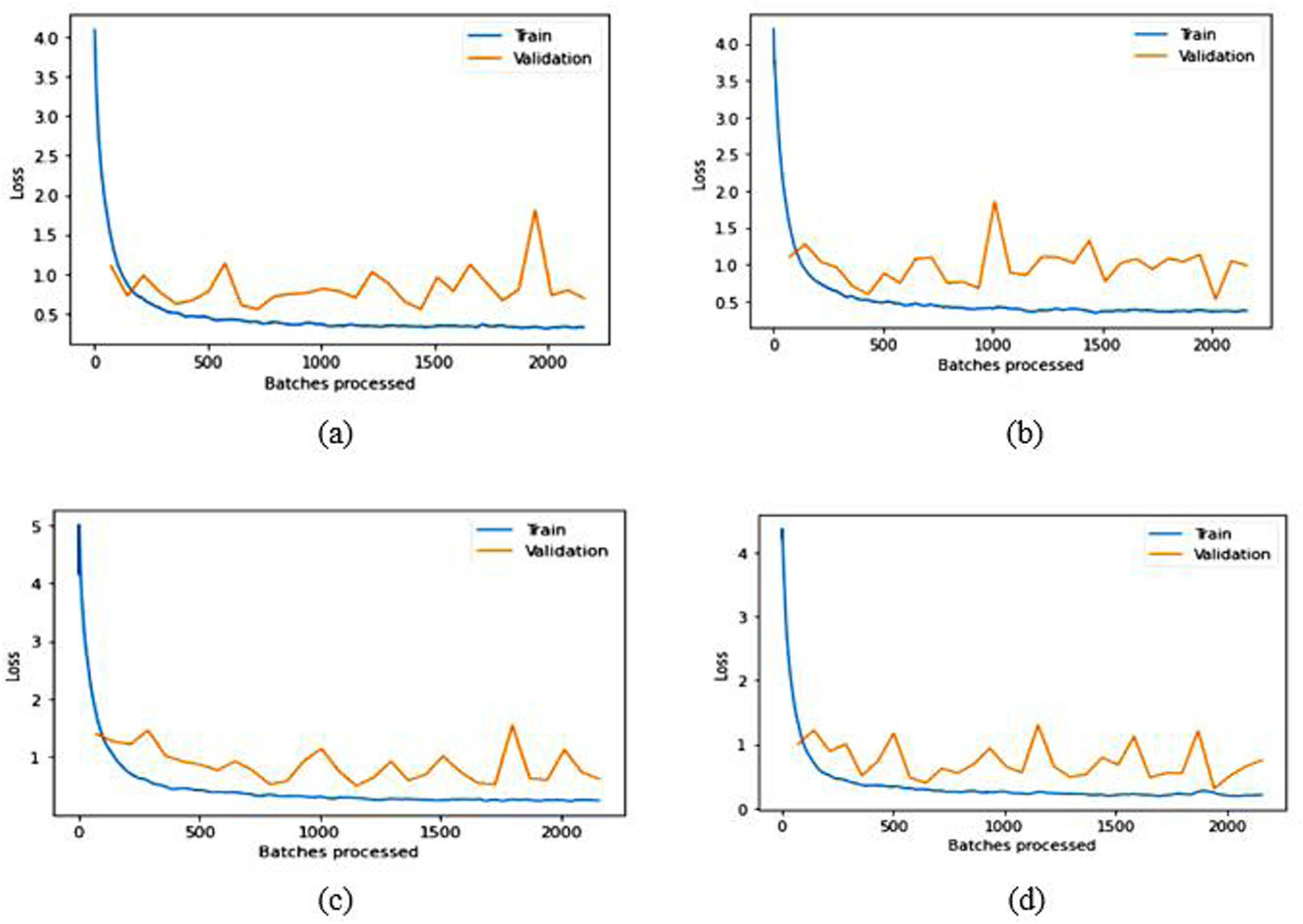
Training and validation loss over batches processed graphs for pre-trained (a) VGG16, (b) VGG19, (c) ResNet50, and (d) DenseNet169 in the LFW dataset.

Figure 9

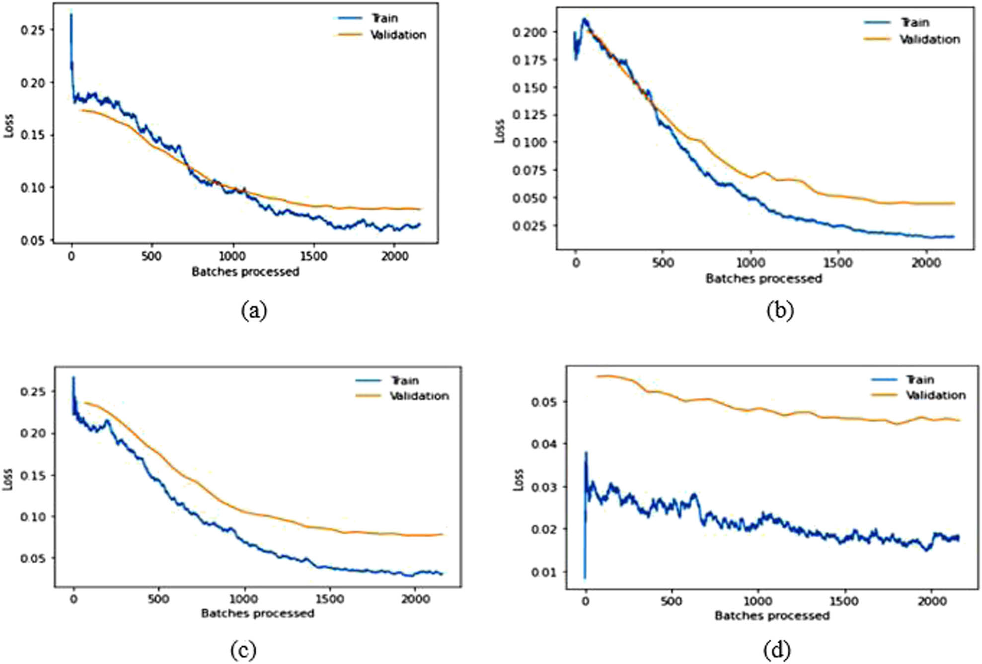
Training and validation loss over batches processed graphs for modified (a) VGG16, (b) VGG19, (c) ResNet50, and (d) DenseNet169 in the LFW dataset.

3.2.2 Experimental results on the CPLFW dataset

In this experimental evaluation, random splitting of the CPLFW dataset is done with a splitting ratio of 8:2 (i.e., 80% of images [9,322] are used for training and 20% [2,330] are used for validating the model). The dropout values are set to 0.25 and 0.5. Training and validation losses for different models are shown in Table 5. The comparison of the proposed approach with other existing techniques is listed in Table 6. Finally, the training and validation loss over batches processed graphs for the pre-trained and fine-tuned baseline models are delineated in Figures 10 and 11.

Table 5

Training and validation loss of pre-trained models (VGG16, VGG19, ResNet50, and DenseNet169) and modified pre-trained models with PC in CPLFW

Model	TH = T/F	E	LR	TL	VL	ER	TA	VA	P	R
Pre-trained models
VGG16	—	15	1 × 10−3	0.1580	0.6419	0.1215	0.9634	0.8784	0.8711	0.8734
VGG19	—	15	1 × 10−3	0.1623	0.6357	0.1280	0.9563	0.8719	0.8654	0.8724
ResNet50	—	15	1 × 10−3	0.0678	0.4507	0.0905	0.9856	0.9094	0.9001	0.9054
DenseNet169	—	15	1 × 10−3	0.0501	0.4378	0.0887	0.9898	0.9112	0.9200	0.9198
Modified pre-trained models with PC
Modified VGG16	T	7	2.75 × 10−2	1.1628	0.9759	0.2077	0.7734	0.7922	0.7792	0.7986
	F	15	6.31 × 10−7, 1 × 10−5	0.8944	0.8895	0.1896	0.8112	0.8103	0.8264	0.8164
Modified VGG19	T	7	1.1 × 10−2	1.4396	1.2920	0.2603	0.7243	0.7396	0.7256	0.7345
	F	15	1 × 10−5, 5 × 10−4	0.2921	0.4468	0.0844	0.9323	0.9155	0.9166	0.9132
Modified ResNet50	T	7	1.32 × 10−2	0.5944	0.6587	0.1314	0.8867	0.8685	0.8764	0.8678
	F	15	2.2 × 10−6, 1 × 10−4	0.2334	0.4462	0.0849	0.9458	0.9150	0.9245	0.9152
Modified DenseNet169	T	7	1.32 × 10−2	0.4330	0.4568	0.0879	0.9198	0.9120	0.9132	0.9134
	F	15	5 × 10−6, 5 × 10−5	0.2227	0.3583	0.0842	0.9289	0.9157	0.9234	0.9219

PC, proposed classifier; TH, Train_head; E, epoch; LR, learning rate; TL, training loss; VL, validation loss; ER, error rate; TA, training accuracy; VA, validation accuracy; P, precision; R, recall.

The bold values mean the best values in comparison to other comparing methods.

Table 6

Comparison of the proposed work with other SOTA in the CPLFW dataset

Author, year of publication	Techniques used	Accuracy (%)	Error rate (%)
Liu et al., 2017 [50]	SphereFace	81.4	18.6
Cao et al., 2018 [51]	VGGFace2	84	16
Liu et al., 2021 [52]	Lightweight CNN	89.52	10.48
Proposed approach	Hybrid model of the fine-tuned pre-trained models using ensemble learning	91.58	8.42

The bold value means the best value in comparison to other methods.

Figure 10

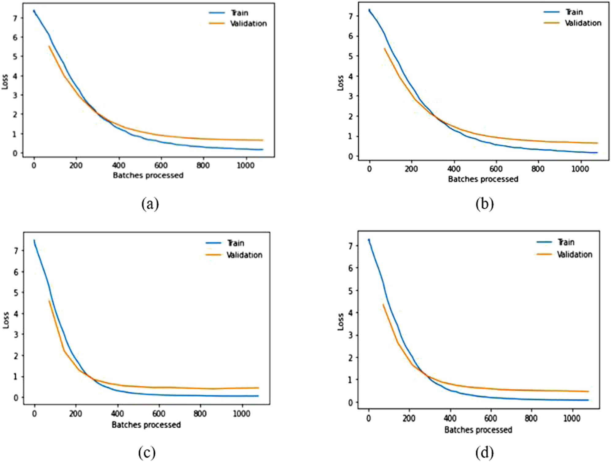
Training and validation loss over batches processed graphs for pre-trained (a) VGG16, (b) VGG19, (c) ResNet50, and (d) DenseNet169 in the CPLFW dataset.

Figure 11

Training and validation loss over batches processed graphs for modified (a) VGG16, (b) VGG19, (c) ResNet50, and (d) DenseNet169 in the CPLFW dataset.

3.2.3 Experimental results on the self-created criminal dataset

A small criminal dataset is created containing 25 images of each class of criminals, namely Haji Mastan, Vijay Mallya, Dawood, Harshad, Osama, Veerappan, Chhota Rajan, Muthappa Rai, Abu Salem, and Vikas Dubey, by downloading these images from the internet to demonstrate the real-time application of face recognition. Mislabeled and vague images from the downloaded images are manually deleted and 25 images of each class are considered to make a class-balanced dataset. Data augmentation, known as the oversampling technique, is utilized to expand the count of samples in each class. In order to maintain the balance of the class, images in individual classes are augmented to generate 50 samples using a set of transformations, such as vertical flip, horizontal flip, mirroring, warping, scaling, rotation, zooming, and lighting. The dataset is divided into two sets consisting of 80 and 20% samples (i.e., 400 samples of the dataset are considered for training and 100 samples are taken for testing). Testing on a self-created dataset is done in two ways. First, the testing is done using 100 random samples from 500 images. The accuracy of the proposed hybrid model on a self-created dataset is 95%, while the precision score, recall score, and error rate are 0.954167, 0.952393, and 5%, respectively. The confusion matrix to analyze the correct results present in the diagonal of the matrix is delineated in Figure 12.

Figure 12

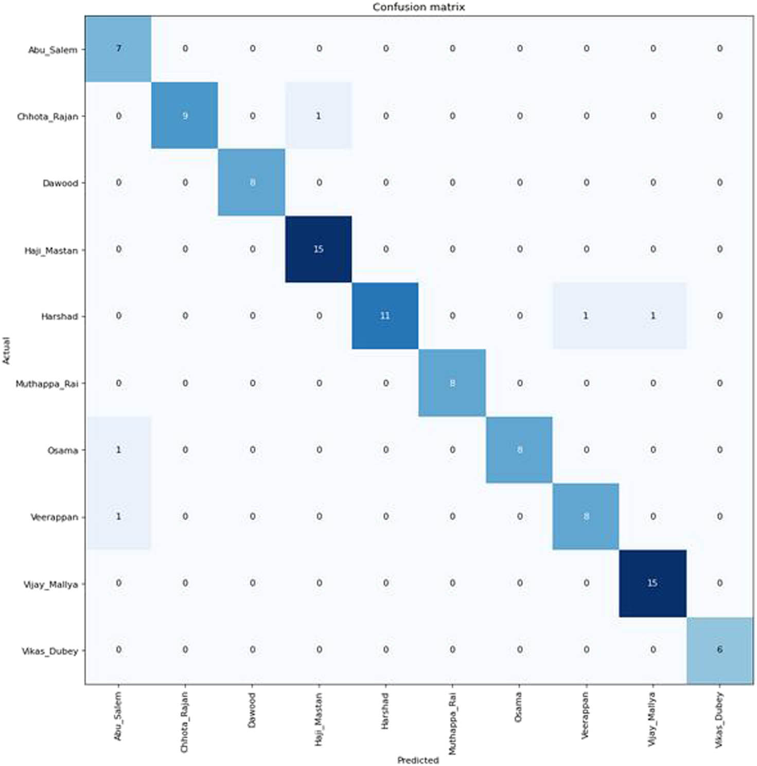
Confusion matrix for the testing of 100 images.

Second, another testing dataset contains 50 images with more than one face to demonstrate the real-time surveillance results. The set of 50 images is distinct from the collection of 500 images but consists of the faces of the same 10 criminals and other unknown individuals. As the testing images contain more than one face, the recognition rate of the proposed technique in the criminal dataset is calculated by manually analyzing each image, as shown in Figure 13, achieving 87% recognition accuracy.

Figure 13

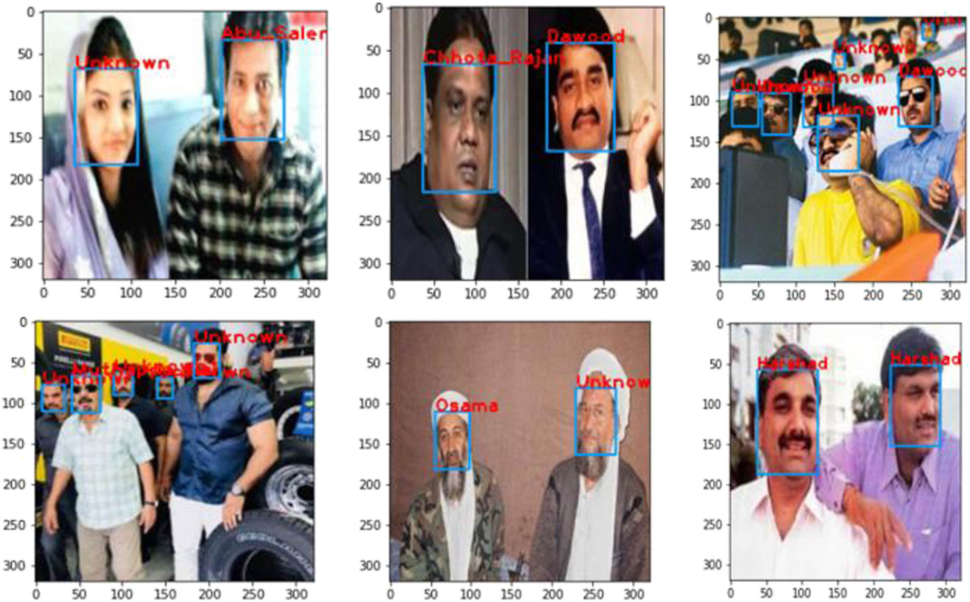
Results of the recognition of criminals in a self-created dataset for testing 50 images.

References

[1] Xiao K, Tian Y, Lu Y, Lai Y, Wang X. Quality assessment-based iris and face fusion recognition with dynamic weight. Vis Comput. 2022;38:1631–43.10.1007/s00371-021-02093-7Search in Google Scholar
[2] Min-Allah N, Jan F, Alrashed S. Pupil detection schemes in human eye: a review. Multimed Syst. 2021 Aug;27(4):753–77.10.1007/s00530-021-00806-5Search in Google Scholar
[3] Kortli Y, Jridi M, Al Falou A, Atri M. Face recognition systems: A survey. Sensors. 2020 Jan 7;20(2):342.10.3390/s20020342Search in Google Scholar PubMed PubMed Central
[4] Kumar Shukla R, Kumar Tiwari A. Comparative analysis of machine learning based approaches for face detection and recognition. J Inf Technol Manag. 2021 Jan 1;13(1):1–21.Search in Google Scholar
[5] Tan C, Sun F, Kong T, Zhang W, Yang C, Liu C. A survey on deep transfer learning. In: Kůrková V, Manolopoulos Y, Hammer B, Iliadis L, Maglogiannis I, editors. Artificial Neural Networks and Machine Learning–ICANN 2018. 27th International Conference on Artificial Neural Networks; 2018 Oct 4–7; Rhodes, Greece. Springer, 2018. p. 270–9.10.1007/978-3-030-01424-7_27Search in Google Scholar
[6] Niu S, Liu Y, Wang J, Song H. A decade survey of transfer learning (2010–2020). IEEE Trans Artif Intell. 2020 Oct;1(2):151–66.10.1109/TAI.2021.3054609Search in Google Scholar
[7] Punia SK, Kumar M, Stephan T, Deverajan GG, Patan R. Performance analysis of machine learning algorithms for big data classification: Ml and ai-based algorithms for big data analysis. Int J E-Health Med Commun (IJEHMC). 2021 Jul 1;12(4):60–75.10.4018/IJEHMC.20210701.oa4Search in Google Scholar
[8] Vaiyapuri T, Mohanty SN, Sivaram M, Pustokhina IV, Pustokhin DA, Shankar K. Automatic vehicle license plate recognition using optimal deep learning model. Comput Mater Continua. 2021 Jan 1;67(2):1881–97.10.32604/cmc.2021.014924Search in Google Scholar
[9] Vetriselvi T, Lydia EL, Mohanty SN, Alabdulkreem E, Al-Otaibi S, Al-Rasheed A, et al. Deep learning based license plate number recognition for smart cities. Comput Mater Continua. 2022 Jan 1;70(1):2049–64.10.32604/cmc.2022.020110Search in Google Scholar
[10] Guo Y, Liu Y, Oerlemans A, Lao S, Wu S, Lew MS. Deep learning for visual understanding: A review. Neurocomputing. 2016 Apr 26;187:27–48.10.1016/j.neucom.2015.09.116Search in Google Scholar
[11] Sun Y, Wang X, Tang X. Deep learning face representation from predicting 10,000 classes. Proceedings of the IEEE Conference on Computer Vision and Pattern Recognition; 2014 Jun 23–28; Columbus (OH), USA. IEEE, 2014. p. 1891–8.10.1109/CVPR.2014.244Search in Google Scholar
[12] Parkhi OM, Vedaldi A, Zisserman A. Deep face recognition. BMVC. 2015;1:6.10.5244/C.29.41Search in Google Scholar
[13] Huang GB, Mattar M, Berg T, Learned-Miller E. Labeled faces in the wild: A database for studying face recognition in unconstrained environments. Workshop on Faces in ‘Real-Life’ Images: Detection, Alignment, and Recognition; 2008 Oct; Marseille, France.Search in Google Scholar
[14] Wolf L, Hassner T, Maoz I. Face recognition in unconstrained videos with matched background similarity. CVPR 2011; 2011; Jun 20–25; Colorado Springs (CO), USA. IEEE, 2011. p. 529–34.10.1109/CVPR.2011.5995566Search in Google Scholar
[15] Wen Y, Zhang K, Li Z, Qiao Y. A discriminative feature learning approach for deep face recognition. In: Leibe B, Matas J, Sebe N, Welling M, editors. Computer Vision–ECCV 2016: 14th European Conference; 2016 Oct 11–14; Amsterdam, The Netherlands. Springer, 2016. p. 499–515.10.1007/978-3-319-46478-7_31Search in Google Scholar
[16] Sagi O, Rokach L. Ensemble learning: A survey. Wiley Interdiscip Reviews: Data Min Knowl Discovery. 2018 Jul;8(4):e1249.10.1002/widm.1249Search in Google Scholar
[17] Tang J, Su Q, Su B, Fong S, Cao W, Gong X. Parallel ensemble learning of convolutional neural networks and local binary patterns for face recognition. Comput Methods Prog Biomed. 2020 Dec 1;197:105622.10.1016/j.cmpb.2020.105622Search in Google Scholar PubMed
[18] Alhanaee K, Alhammadi M, Almenhali N, Shatnawi M. Face recognition smart attendance system using deep transfer learning. Procedia Comput Sci. 2021 Jan 1;192:4093–102.10.1016/j.procs.2021.09.184Search in Google Scholar
[19] Ganaie MA, Hu M, Malik AK, Tanveer M, Suganthan PN. Ensemble deep learning: A review. Eng Appl Artif Intell. 2022 Oct 1;115:105151.10.1016/j.engappai.2022.105151Search in Google Scholar
[20] Fayek HM, Cavedon L, Wu HR. Progressive learning: A deep learning framework for continual learning. Neural Netw. 2020 Aug 1;128:345–57.10.1016/j.neunet.2020.05.011Search in Google Scholar PubMed
[21] Barreto S. What is Fine-tuning in Neural Networks?; 2022. https://www.baeldung.com/cs/fine-tuning-nn. Accessed on 24 March 2023.Search in Google Scholar
[22] Lin M, Chen Q, Yan S. Network in network. arXiv preprint. arXiv:1312.4400; 2013 Dec 16.Search in Google Scholar
[23] Basha SS, Dubey SR, Pulabaigari V, Mukherjee S. Impact of fully connected layers on performance of convolutional neural networks for image classification. Neurocomputing. 2020 Feb 22;378:112–9.10.1016/j.neucom.2019.10.008Search in Google Scholar
[24] Ioffe S, Szegedy C. Batch normalization: Accelerating deep network training by reducing internal covariate shift. In: Bach F, Blei D, editors. International Conference on Machine Learning; 2015 Jul 6–11; Lille, France. ACM, 2015. p. 448–56.Search in Google Scholar
[25] Srivastava N, Hinton G, Krizhevsky A, Sutskever I, Salakhutdinov R. Dropout: a simple way to prevent neural networks from overfitting. J Mach Learn Res. 2014 Jan 1;15(1):1929–58.Search in Google Scholar
[26] Liu W, Anguelov D, Erhan D, Szegedy C, Reed S, Fu CY, et al. SSD: Single Shot MultiBox Detector. In: Leibe B, Matas J, Sebe N, Welling M, editors. Computer Vision–ECCV 2016: 14th European Conference; 2016 Oct 11–14; Amsterdam, The Netherlands. Springer, 2016. p. 21–37.10.1007/978-3-319-46448-0_2Search in Google Scholar
[27] Zhang K, Zhang Z, Li Z, Qiao Y. Joint face detection and alignment using multitask cascaded convolutional networks. IEEE Signal Process Lett. 2016 Aug 26;23(10):1499–503.10.1109/LSP.2016.2603342Search in Google Scholar
[28] Viola P, Jones MJ. Robust real-time face detection. Int J Comput Vis. 2004 May;57:137–54.10.1023/B:VISI.0000013087.49260.fbSearch in Google Scholar
[29] Ahonen T, Hadid A, Pietikainen M. Face description with local binary patterns: Application to face recognition. IEEE Trans Pattern Anal Mach Intell. 2006 Oct 30;28(12):2037–41.10.1109/TPAMI.2006.244Search in Google Scholar PubMed
[30] Zheng T, Deng W. Cross-pose LFW: A database for studying cross-pose face recognition in unconstrained environments. Beijing Univ Posts Telecommun Tech Rep. 2018 Feb;5(7):1–6.Search in Google Scholar
[31] He K, Zhang X, Ren S, Sun J. Deep residual learning for image recognition. Proceedings of the IEEE Conference on Computer Vision and Pattern Recognition; 2016 Jun 27-30; Las Vegas (NV), USA. IEEE, 2016. p. 770–8.10.1109/CVPR.2016.90Search in Google Scholar
[32] Simonyan K, Zisserman A. Very deep convolutional networks for large-scale image recognition. arXiv preprint. arXiv:1409.1556; 2014 Sep 4.Search in Google Scholar
[33] Huang G, Liu Z, Van Der Maaten L, Weinberger KQ. Densely connected convolutional networks. Proceedings of the IEEE Conference on Computer Vision and Pattern Recognition; 2017 Jul 21–26; Honolulu (HI), USA. IEEE, 2017. p. 2261–9.10.1109/CVPR.2017.243Search in Google Scholar
[34] Russakovsky O, Deng J, Su H, Krause J, Satheesh S, Ma S, et al. Imagenet large scale visual recognition challenge. Int J Comput Vis. 2015 Dec;115:211–52.10.1007/s11263-015-0816-ySearch in Google Scholar
[35] Garbin C, Zhu X, Marques O. Dropout vs batch normalization: an empirical study of their impact to deep learning. Multimed Tools Appl. 2020 May;79:12777–815.10.1007/s11042-019-08453-9Search in Google Scholar
[36] Nair V, Hinton GE. Rectified linear units improve restricted Boltzmann machines. In: Fürkranz J, Joachims T, editors. Proceedings of the 27th International Conference on Machine Learning (ICML-10); 2010 Jun 21–24; Haifa, Israel. ACM, 2010. p. 807–14.Search in Google Scholar
[37] He K, Zhang X, Ren S, Sun J. Delving deep into rectifiers: Surpassing human-level performance on imagenet classification. Proceedings of the IEEE International Conference on Computer Vision; 2015 Dec 7–13; Santiago, Chile. IEEE, 2015. p. 1026–34.10.1109/ICCV.2015.123Search in Google Scholar
[38] Maas AL, Hannun AY, Ng AY. Rectifier nonlinearities improve neural network acoustic models. In: Dasgupta S, McAllester D, editors. Proceedings of the 30th International conference on Machine Learning; 2013 Jun 16–21; Atlanta (GA), USA. Search in Google Scholar
[39] Smith LN. Cyclical learning rates for training neural networks. 2017 IEEE Winter Conference on Applications of Computer Vision (WACV); 2017 Mar 24-31; Santa Rosa (CA), USA. IEEE, 2017. p. 464–72.10.1109/WACV.2017.58Search in Google Scholar
[40] Kingma DP, Ba J. Adam: A method for stochastic optimization. arXiv preprint. arXiv:1412.6980; 2014 Dec 22.Search in Google Scholar
[41] Brownlee J. How to Develop a Weighted Average Ensemble With Python; 2021. https://machinelearningmastery.com/weighted-average-ensemble-with-python/ (accessed March 25th, 2023).Search in Google Scholar
[42] Venu SK. An ensemble-based approach by fine-tuning the deep transfer learning models to classify pneumonia from chest X-ray images. arXiv preprint. arXiv:2011.05543; 2020 Nov 11.Search in Google Scholar
[43] Bradski G. The openCV library. Dr Dobb’s J Softw Tools Prof Program. 2000;120:122–5.Search in Google Scholar
[44] Branco P, Torgo L, Ribeiro RP. A survey of predictive modeling on imbalanced domains. ACM Comput Surv (CSUR). 2016 Aug 13;49(2):1–50.10.1145/2907070Search in Google Scholar
[45] Afonja T. Accuracy Paradox; 2017. https://towardsdatascience.com/accuracy-paradox-897a69e2dd9b Accessed on 13 April 2022.Search in Google Scholar
[46] Perez L, Wang J. The effectiveness of data augmentation in image classification using deep learning. arXiv preprint. arXiv:1712.04621; 2017 Dec 13.Search in Google Scholar
[47] Kang K. Comparison of face recognition and detection models: Using different convolution neural networks. Optical Mem Neural Netw. 2019 Apr;28:101–8.10.3103/S1060992X19020036Search in Google Scholar
[48] Ben Fredj H, Bouguezzi S, Souani C. Face recognition in unconstrained environment with CNN. Vis Comput. 2021 Feb;37:217–26.10.1007/s00371-020-01794-9Search in Google Scholar
[49] Mishra NK, Singh SK. Regularized Hardmining loss for face recognition. Image Vis Comput. 2022 Jan 1;117:104343.10.1016/j.imavis.2021.104343Search in Google Scholar
[50] Liu W, Zhang YM, Li X, Yu Z, Dai B, Zhao T, Song L. Deep hyperspherical learning. Adv Neural Inf Process Syst. 2017;30:1–11.Search in Google Scholar
[51] Cao Q, Shen L, Xie W, Parkhi OM, Zisserman A. VGGFace2: A dataset for recognising faces across pose and age. 2018 13th IEEE International Conference on Automatic Face & Gesture Recognition (FG 2018); 2018 May 15–19; Xi'an, China. IEEE, 2018. p. 67–74.10.1109/FG.2018.00020Search in Google Scholar
[52] Liu W, Zhou L, Chen J. Face recognition based on lightweight convolutional neural networks. Information. 2021 Apr 28;12(5):191.10.3390/info12050191Search in Google Scholar
© 2023 the author(s), published by De Gruyter
This work is licensed under the Creative Commons Attribution 4.0 International License.